
Documents Live, a web authoring and publishing system
If you see this, something is wrong
Table of contents
First published on Friday, Mar 28, 2025 and last modified on Thursday, Apr 10, 2025 by François Chaplais.
Published version: 10.48550/arXiv.2503.20772
Automatic Control Laboratory, ETH Zurich, 8092 Zurich, Switzerland Email
Automatic Control Laboratory, ETH Zurich, 8092 Zurich, Switzerland Email
Automatic Control Laboratory, ETH Zurich, 8092 Zurich, Switzerland Email
Zurich Center for Market Design & SUZ, University of Zurich, 8050 Zurich, Switzerland Email
Automatic Control Laboratory, ETH Zurich, 8092 Zurich, Switzerland Email
Abstract
Many multi-agent socio-technical systems rely on aggregating heterogeneous agents’ costs into a social cost function (SCF) to coordinate resource allocation in domains like energy grids, water allocation, or traffic management. The choice of SCF often entails implicit assumptions and may lead to undesirable outcomes if not rigorously justified. In this paper, we demonstrate that what determines which SCF ought to be used is the degree to which individual costs can be compared across agents and which axioms the aggregation shall fulfill. Drawing on the results from social choice theory, we provide guidance on how this process can be used in control applications. We demonstrate which assumptions about interpersonal utility comparability – ranging from ordinal level comparability to full cardinal comparability – together with a choice of desirable axioms, inform the selection of a correct SCF, be it the classical utilitarian sum, the Nash SCF, or maximin. We then demonstrate how the proposed framework can be applied for principled allocations of water and transportation resources.
1 Introduction
Multi-agent socio-technical control applications with heterogeneous agents arise in various domains, such as energy grids, traffic control, water distribution, and bandwidth allocation [1]. In these systems, the control objective in the form of a social cost function (SCF) is typically context-specific, and it often involves some cost or utility aggregation across agents, reflecting agents’ different goals, needs, and operational constraints. When performance indicators (e.g., energy consumption, travel time, bandwidth usage) are measurable and objective, one might sometimes quite straightforwardly design an SCF such as total cost or throughput. However, when agents’ costs represent subjective, agent-specific valuations, it is often unclear if these costs can be compared objectively, leading to difficulties and ambiguities in aggregating these costs and defining SCFs.
Several candidate SCFs, including the sum (or weighted sum) of utilities/costs, Nash social cost, and max-min objectives, exist in the literature [2, 3, 4, 5], with the choice among these criteria usually depending on desired properties such as tractability, fairness, and robustness. A most popular approach to aggregate individual costs is the classical utilitarian rule, which sums individual costs into a single objective. While intuitive and computationally tractable, this approach assumes that the cost for one agent is commensurate with the cost of another. In practice, this is a strong comparability assumption which can lead to unintended consequences [6], e.g., disproportionally high wait times for ride-hails in remote areas [7], discrimination against certain train types or routes in real-time train re-scheduling [8], or exacerbation of energy poverty [9].
Exact full comparability of the costs incurred by different agents can be impeded by various reasons. In some cases, it is an issue of measurability, i.e., it might be difficult to precisely estimate costs because they depend on complex models and unknown parameters (e.g., the yield of a farm as a function of the water allocated to it or the delay incurred outside the traffic network of interest). In some cases, the decision maker cannot compare the subjective evaluation of the costs incurred by an agent (e.g., the value of travel time, which depends on socio-economic and circumstantial factors[10, 11]). In other cases, costs are self-reported and therefore vulnerable to strategic manipulation (e.g., customers declaring their electricity needs [12]). Finally, limited comparability of agents’ costs may encode fairness criteria, as it defines what information about the agents’ preferences should be considered in the decision (e.g., a deliberate decision on whether a traffic congestion protocol should prioritize vehicles that have accumulated delay).
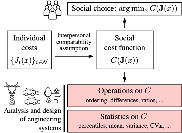
The central aim of this paper is to offer an axiomatic viewpoint on how to properly aggregate agents’ costs in multi-agent decision and control depending on their comparability. By reviewing, adapting, and extending the main concepts of welfarism and interpersonal comparability to the specific context of multi-agent control, this paper develops and recommends a design procedure that comprises the following steps (Figure 1):
- Determine the level of interpersonal comparability. Such a decision is guided by the measurability and comparability of the agents’ preferences but it can also be a deliberate decision guided by politics, social agreements, and public sentiment.
- Select the appropriate social cost function. Based on the selected comparability level, a restricted choice of possible SCFs is allowed. We provide rigorous guarantees about its robustness with respect to the lack of measurability and comparability.
- Apply social cost function. Given an appropriate control, decision or optimization problem, the selected SCF can be explicitly optimized to select the best social choice, or can be used to for the analysis and design of these engineering systems. We provide rigorous guarantees about the set of permissible operations.
We expect these results to be relevant in many control applications where specifications are provided in the form of social cost/welfare function [13]. The mathematical guarantees that we provide can be incorporated in the design of system-wide metrics that are now being used in multi-agent control, like Price of Anarchy [14, 15, 16, 17, 18]. They can also guide the design of optimization dynamics [19, 20, 21] and resource allocation mechanisms [22, 23]. Finally, our work responds to the growing interest in fairness in control [1, 24, 25, 26, 27, 28], as many fairness notions arise naturally from careful considerations of the level of interpersonal comparability.
The aforementioned three-step procedure can also be interpreted in reverse, especially when designing engineering systems: if a specific notion of efficiency/fairness is desired (utilitarian, min/max, etc.) then a sufficient level of comparability needs to be achieved, which may require the collection of additional information from the agents, the design of a manipulation-safe mechanism, or the use of more accurate cost models. This may give a principled perspective on how freely agents’ costs can be designed and engineered [29, 30, 31].
The remainder of this paper is structured as follows. In Section 2, we introduce desirable axioms that will set the stage for a principled welfarist approach based on social choice theory [32, 33, 34]. In Section 3, we derive results on how desirable axioms, together with limits/possibilities of interpersonal cost comparability, determine which social cost aggregations are permissible. In Section 4, we illustrate the versatility of the proposed framework via examples from water distribution and transportation.
2 Welfarism
In this section we introduce preliminaries adopted from social choice theory that allow a rigorous aggregation of individual costs and derivation of social cost functions. We lay out the foundations of a so called ‘welfarist’ approach, that requires that all the relevant information for the social decision is contained in the agents’ cost functions.
2.1 Preliminaries and Axiomatic Foundations
Let \( \mathcal{N} = \{1,2,\dots,n\}\) be a finite set of agents and let \( \mathcal{X}\) denote the set of feasible outcomes \( x\) . An outcome can be a specific allocation of a scarce resource or any control decision that affects the agents. Each agent \( i \in \mathcal{N}\) is endowed with a preference relation \( \succsim_i\) over \( \mathcal{X}\) . We assume that \( \succsim_i\) is complete and transitive . Under mild regularity conditions, these preferences can be represented by a real-valued cost function defined on \( \mathcal{X}\) . Thus we let \( J_i(\cdot) \in \mathcal{J}\) , where \( \mathcal{J}\) is the set of all real-valued functions on \( \mathcal X\) , denote the cost of agent \( i\) associated with an outcome \( x\) , satisfying
If \( J_i\) additionally satisfies appropriate continuity conditions, we say each agent’s preferences are numerically representable or cardinalizable. We let \( \mathbf{J}=(J_1,\dots,J_n)\) denote a profile of such costs for the entire set of agents. When formulating a resource allocation problem that depends on agents’ individual evaluations represented by \( \mathbf{J}\) , one needs to define a single social preference relation \( \succsim_{\mathbf{J}}\) on \( \mathcal{X}\) , so as to capture the collective or “social” viewpoint. We want to define a mapping between cost profiles and the resulting social preference, which can be expressed using Social Cost Functionals (SCFL):
Definition 1
Let \( \mathcal{R}\) be the set of all complete and transitive binary relations on \( \mathcal{X}\) . A Social Cost Functional (SCFL) is a mapping
such that, for each profile \( \mathbf{J}=(J_1,\dots,J_n)\in \mathcal{J}^n\) , it assigns a social preference relation \( \succsim_{\mathbf{J}} = \mathfrak{F}(\mathbf{J})\) on \( \mathcal{X}\) .
Before determining how to incorporate each agent’s evaluation into a collective decision, one should first specify which fundamental properties (or axioms) this social preference relation \( \succsim_{\mathbf{J}}\) needs to satisfy. Two classical well-established properties that can be expected from such a relation are:
Axiom 1 (Weak Pareto Principle (P))
For any profile \( \mathbf{J}\) and any \( x,y\in \mathcal{X}\) , if \( J_i(x) < J_i(y)\text{ for all }i\) then \( x \succ_{\mathbf{J}} y\) .
Axiom 2 (Independence of Irrelevant Alternatives (IIA))
For any two distinct outcomes \( x,y\in\mathcal{X}\) and any two profiles \( \mathbf{J},\mathbf{J}'\in\mathcal{J}^n\) such that \( J_i(x)=J_i'(x)\) and \( J_i(y)=J_i'(y)\) for each \( i\) , we require
In other words, changing the costs of other outcomes does not affect the pairwise social ranking of \( x\) and \( y\) .
In control applications, it is convenient to work with real-valued measures of social cost rather than a social ordering of outcomes. This requires an additional mild continuity assumption on the SCFL, which postulates that if an outcome \( x\) is socially strictly preferred over \( y\) , it should remain so under a small enough perturbation of the individual costs. As we show in Section 3.2, this condition is easily verified for the setting considered in this work.
Definition 2 (Pairwise Continuity (PC))
For every \( \varepsilon \in \mathbb{R}_{++}^N\) , there exists \( \varepsilon' \in \mathbb{R}_{++}^N\) such that for every profile \( \mathbf{J}\) and every pair \( x,y \in \mathcal X\) with \( x\,\succ_{\mathbf{J}}\,y\) , there exists a profile \( \tilde{\mathbf{J}}\) satisfying \( \tilde{\mathbf{J}}(x) \geq \mathbf{J}(x) + \varepsilon'\) and \( \tilde{\mathbf{J}}(y) \leq \mathbf{J}(y) + \varepsilon\) , and such that \( x\,\succ_{\tilde{\mathbf{J}}}\,y.\)
In some cases it may be desirable to enforce an additional axiom that does not allow to distinguish individual agents.
Axiom 3 (Anonimity (A))
Let \(\pi: \mathbb{N} \to \mathbb{N}\) be a permutation (i.e., a bijection on \(\mathbb{N}\)). If, for all \(i \in \mathbb{N}\) and \(x \in X\), \( J'_i(x) = J_{\pi(i)}(x)\) then \( \succsim_{\mathbf{J}} = \succsim_{\mathbf{J}'}\) .
2.2 Welfarism
If we accept these axioms (P) and (IIA) as reasonable and impose them on our social preference relation, together with condition (PC), we can establish a welfarist principle [35, 32], that implies that any complete and transitive social ordering can be expressed through a Social Cost Function (SCF) \( C\) , which subsumes all relevant information for the ordering.
Lemma 1 (Welfarism; Thm 3.7, [34], Thm 1, [33])
Let \( \succsim_{\mathbf{J}}\) be a social preference relation on \( \mathcal{X}\) defined by SCFL \( \mathfrak{F}\) for any profile \( \mathbf{J}=(J_1,\dots,J_n) \in \mathcal{J}^n\) . Suppose \( \succsim_{\mathbf{J}}\) satisfies (P), (IIA) and (PC). Then there exists a continuous Social Cost Function (SCF)
such that for any \( x,y\in\mathcal{X}\) ,
The SCF \( C\) thus represents the SCFL \( \mathfrak{F}\) and all relevant information for ranking outcomes is contained in the \( n\) -tuple \( \bigl(J_1(x),\dots,J_n(x)\bigr)\) . The welfarist approach thus states that once \( \mathbf{J}\) and the feasible set \( \mathcal{X}\) are specified, the social preference depends only on the vector of costs for each outcome. Any other features of \( x\) or \( y\) are irrelevant from the perspective of the social ordering.
As mentioned in the introduction, several well-known examples of SCFs \( C\) have been proposed to aggregate individual costs. For instance, the utilitarian approach, often attributed to Bentham [36] as later formalized by Harsanyi [37], aggregates costs via a sum: \( C_{\mathrm{util}}(J_1,\dots, J_n)=\sum_{i=1}^n J_i\) . By contrast, the Rawlsian or min-max rule, inspired by Rawls [38], focuses on the well-being of the worst-off agent: \( C_{\mathrm{rawls}}=\max_{i\in\mathcal{N}} J_i\) . Another example is the Nash Social Welfare function [39, 40], which is defined as \( C_{\mathrm{Nash}}(u_1,\dots,u_n)=-\prod_{i=1}^n (-J_i)\) . Typically, selecting a SCF as the objective in a control problem is driven by the desired properties, such as efficiency, fairness, or equity, that the designer wishes to achieve. The focus of this work is to provide a principled way to make this choice based on the fundamental assumptions of interpersonal comparability of the agents’ costs, from which the appropriate aggregation rule naturally follows.
3 Cost Aggregation and Comparability
The welfarist principle (Lemma 1) tells us that any social ordering under (P), (IIA) and (PC) must be representable by a SCF that depends solely on the costs incurred by the agents. One must still decide which \( C\) is appropriate in practice. Such a choice needs to be guided by a deliberate decision on how individual costs can be measured and compared across agents, so that meaningful interpersonal trade-offs can be made in the social choice. Addressing the interpersonal comparability issue corresponds to deciding which transformations of the individual costs leave the social ranking unchanged [32, 33]. By restricting or expanding the class of invariance transformations of the individual costs, one effectively selects a level of measurability and comparability for the agents’ costs. Once the comparability assumptions are fixed, the shape of the SCF \( C\) is essentially pinned down.
This section formalizes these invariance principles and shows how each comparability assumption leads to distinct classes of SCFs.
3.1 Comparability Levels
Definition 3 (Invariance Transformations under a SCF)
Let \( C: \mathcal{X} \to \mathbb{R}\) be a social cost function defined on a set of outcomes \( \mathcal{X}\) . A vector of transformations \( \{\phi_i \in \Phi : i \in \mathcal{N}\}\) is called an invariance transformation under \( C\) if, for any cost profile \( \mathbf{J}=(J_1,\dots,J_n)\) , the transformed profile
is equivalent to \( \mathbf{J}\) under \( C\) , meaning that for all \( x,y \in \mathcal{X}\) ,
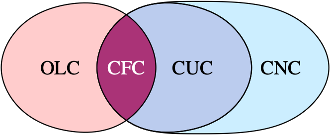
We present four levels of interpersonal comparability, defined via the corresponding invariance transformations. Notice that by imposing a specific invariance condition on the SCF \( C\) , we are equivalently defining an information filter that specifies what features of the individual cost profiles are relevant for the social ordering. For each comparability level, we comment on what kind of equivalence they induce on the costs \( J_i\) in terms of measurability and comparability.
- Ordinal Level Comparability (OLC).
The costs \( J_i\) are determined up to any common strictly increasing transformation \( \phi_{\text{ OLC}}\) :
\[ J_i'(x) = \phi_{\text{ OLC}}\bigl(J_i(x)\bigr) \]We cannot compare cost increments, but it is possible to order the costs incurred by different agents.
- Cardinal Non-Comparability (CNC).
The costs \( J_i\) are determined up to distinct positive affine transformations:
\[ J_i'(x) = \phi_{\text{ CNC}}(J_i(x)) := a_i\,J_i(x) \;+\; b_i, ~ a_i>0, \]i.e., each agent has its own scale and origin. We can compare increments within a single agent’s cost, but we cannot compare costs or increments across agents.
- Cardinal Unit Comparability (CUC).
The costs \( J_i\) are determined up to any common scale factor \( a\) , but may have distinct offsets \( b_i\) :
\[ J_i'(x) = \phi_{\text{ CUC}} (J_i(x)) := a\,J_i(x) \;+\; b_i, ~ a>0, \]We can compare increments in cost across agents; however, absolute costs across agents are not comparable.
- Cardinal Full Comparability (CFC).
The costs \( J_i\) are determined up to common positive affine transformations:
\[ J_i'(x) = \phi_{\text{ CFC}} (J_i(x)) := a\,J_i(x) \;+\; b, ~ a>0. \]All agents share a single absolute scale, so both cost levels and increments are comparable.
Figure 2 illustrates the hierarchy of these comparability levels. One should carefully consider what comparability level and associated invariance condition are justified in a given socio-technical control setting. Too little comparability may prevent meaningful trade-offs, whereas too much comparability might overstate the legitimacy of comparisons across agents whose costs are inherently heterogeneous.
3.2 Permissible Social Cost Functions

Classical results in the literature — most notably by Sen [41, 35], d’Aspremont and Gevers [34], and Roberts [33] — demonstrate that if a Social Cost Functional (SCFL) satisfies (P) and (IIA), then its form is uniquely determined by the level of interpersonal comparability assumed. We first provide a technical result informally stated in [42], then formalize the SCF choice in Theorem 1, summarizing results from the literature above in the formalism of our paper (see Figure 3 for a visual guide).
Lemma 2
(OLC), (CNC), (CUC), (CFC) imply Pairwise Continuity (PC).
Proof
Let \( \varepsilon=(\varepsilon_1,\dots,\varepsilon_n)\in\mathbb{R}_{++}^n\) . Since, under (OLC), (CNC), (CUC), and (CFC), \( \mathfrak F\) is invariant under constant shifts \( J_i(x)\to J_i(x)+\alpha_i\) (with \( \alpha_i\) independent of \( x\) and \( \varepsilon' = \max_i \varepsilon_i\) for (CFC)), choose \( \alpha_i=\varepsilon_i\) for all \( i\) and define
Then, for any \( x,y\in \mathcal X\) with \( x\succ_{\mathbf{J}} y\) , invariance yields \( x\succ_{\tilde{\mathbf{J}}} y\) and, since the shift is uniform in \( x\) , the (PC) condition holds with \( \varepsilon'=\varepsilon\) .
Theorem 1 (Choice of Social Cost Functions [33], [34])
Let \( \mathfrak{F} : \mathcal{J}^n \to \mathcal{R}\) be a Social Cost Functional satisfying (IIA) \( +\) (P) (unless stated otherwise). We have the following results, for each level of interpersonal comparability.
- (OLC):
The SCFL \( \mathfrak{F}\) is represented by the SCF
\[ C(\mathbf{J}(x)) \;=\; \max_{i\in\mathcal{N}} J_i(x). \] - (CNC):
A SCFL that satisfies the axioms does not exist. However, if we assume Partial Independence (PI) instead of (IIA), then the SCFL \( \mathfrak{F}\) is represented by the SCF
\[ C(\mathbf{J}(x)) \;=\; -\prod_{i\in\mathcal{N}} \Bigl[J_i(x_0) - J_i(x)\Bigr]^{c_i}, ~~ c_i>0. \]where \( x_0\) is a fixed benchmark outcome such that \( J_i(x_0) \ge J_i(x)\) for all \( x\) .
- (CNC with \( b_i=0\) ):
If all costs \( J_i\) are strictly negative then the SCFL \( \mathfrak{F}\) is represented by the SCF
\[ C(\mathbf{J}(x)) \;=\; -\prod_{i\in\mathcal{N}} \Bigl[\,-J_i(x)\Bigr]^{c_i}, ~~ c_i>0. \] - (CUC):
The SCFL \( \mathfrak{F}\) is represented by the SCF
\[ C(\mathbf{J}(x)) \;=\; \sum_{i\in\mathcal{N}} c_i\,J_i(x), ~~ c_i>0. \] - (CFC):
The SCFL \( \mathfrak{F}\) is represented by the SCF
\[ \!C(\mathbf{J}(x)) = \frac{1}{n}\sum_{i\in\mathcal N} J_i(x)\;+\; g\left( \left[\begin{smallmatrix} J_1(x) - \frac{1}{n}\sum_{i\in\mathcal N} {J}(x) \\ \vdots \\ J_n(x) - \frac{1}{n}\sum_{i\in\mathcal N} {J}(x) \end{smallmatrix}\right] \right) \]with \( g: \mathbb R^n \to \mathbb R\) homogeneous of degree 1. For example one could choose \( \gamma \max(\cdot)\) with \( 0 \leq \gamma \leq 1\) , thus reflecting a balance between efficiency and equity.
Additionally, if one requires the axiom of Anonymity (A), then all the \( c_i\) become equal, i.e. \( c_i = c_j, \forall i,j \in \mathcal{N}\) , and the function \( g\) must be invariant to permutations of the agents.
| Comparability | OLC | CNC | CUC | CFC |
| Invariant tf. | incr. \( \phi_\text{OLC}(J_i)\) | \( \phi_{\text{ CNC}}(J_i) = a_i J_i + b_i\) | \( \phi_{\text{ CUC}}(J_i) = a J_i + b_i\) | \( \phi_{\text{ CFC}}(J_i) = a J_i + b\) |
| SCF \( C(x)\) | \( \max_{i} J_i(x)\) | \( - \prod_{i} \left[J_i(x_0) - J_i(x)\right]^{c_i}\) with benchmark \( x_0\) \( -\prod_{i} \left[ -J_i(x) \right]^{c_i}\) with \( b_i=0\) and negative costs | \( \sum_{i} c_i\,J_i(x)\) | \( \frac{1}{n}\sum_{i} J_i(x)\;+\; g\left(
\left[\begin{smallmatrix}
J_1(x) - \frac{1}{n}\sum_{i} {J}(x) \\
\vdots \\
J_n(x) - \frac{1}{n}\sum_{i} {J}(x)
\end{smallmatrix}\right]
\right)\) \( g\) homogeneous of degree 1 |
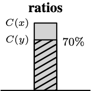
| Allowed operations on the SCF \( C(x)\) | 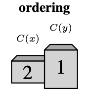 |
 |
 | |
3.3 Admissible Operations on Social Cost Functions
In many engineering problems, one is interested in using the social cost function to guide other operations rather than minimizing it to select the optimal outcome (Figure 1). For example, it may be necessary to perform a quantitative comparison between two possible outcomes (that is, not necessarily selecting the optimal one, but also assessing relative performances). Moreover, in stochastic settings, it may be necessary to compute some statistics on the value of the SCF, like estimating confidence intervals and percentiles, means, variance, or other quantities useful in risk assessment and stochastic optimization.
One needs to be particularly careful about using SCFs for these purposes because Lemma 1 only certifies their use for selecting the best social choice. It is allowed, however, to perform other operations on the values of SCF for different outcomes, as long as the result of such operations is invariant with respect to the transformations listed in Section 3.1, which guarantees that the result of such operations is meaningful. The following lemma allows us to characterize the set of operations that satisfy this property in Proposition 1.
Lemma 3
Consider \( n\) values \( (w_1,\dots,w_n) \in \mathbb{R}^n\) . Suppose \( q(w_1,\dots,w_n)\) is a rational function satisfying \( \forall\,a \in \mathbb{R}_{++},\;\forall\,b \in \mathbb{R}\)
Then \( q\) is a rational function of the ratios of differences:
Conversely, any rational expression built from these ratios of differences is invariant under \( t \mapsto a\,t + b\) .
Proof
First, \( \forall w_i\) define transformation \( w_i \mapsto a\,w_i + b\) as an action of an affine group \( \mathrm{Aff}(1,\mathbb{R})= \{A_{a,b} : t \mapsto a\,t + b \mid a \in \mathbb{R}_{++}, \,b \in \mathbb{R} \}.\) Each affine transformation \( t \mapsto a\,t + b\) can be represented by the matrix \( \left[\begin{smallmatrix} a & b \\ 0 & 1 \end{smallmatrix}\right]\) in a general linear group \( \mathrm{GL}_2(K)\) , acting on row vectors \( (t,1)\) by right multiplication. Hence we have an injective group homomorphism \( \mathrm{Aff}(1,K) \;\hookrightarrow\; \mathrm{GL}_2(K).\) Embed each \( w_i\) in \( \mathbb{R}^2\) (or in another words, embed each \( w_i\) into projective space \( \mathbf{P}^1\) via homogeneous coordinates) by writing \( w_i := (\,w_i,\;1\,)\) . Thus, affine transformations can be seen as the action of a subgroup of \( \mathrm{GL}_2(K)\) on the pairs \( (w_i,1)\) . Now consider the polynomial ring of pairs of variables \( K[x_1,y_1,\;\dots,\;x_n,y_n]\) over an infinite field \( K\) and its quotient field \( K(x,y)\) . Denote the corresponding invariant field by \( K(x, y )^{GL_2}\) . Set \( f_{i,j} := x_iy_j - y_ix_j, 1 \leq i<j \leq n.\) The First Fundamental Theorem for \( GL_2(K)\) [43] states that under the natural \( \mathrm{GL}_2(K)\) action all invariant rational functions lie in the field generated by the ratio-invariants \( \tfrac{f_{i,j}}{\,f_{k,\ell}\,}\) , that is:
Substituting pair of variables for the embedded representation \( (x_i,y_i)=(w_i,1)\) into \( f_{i,j}\) , i.e. expressing them as \( f_{i,j} =x_i\,y_j - y_i\,x_j = w_i - w_j\) , together with the fact that \( \mathrm{Aff}(1, \mathbb{R})\) is a subgroup of \( GL_2(\mathbb{R})\) gives us the result:
Proposition 1 (Invariance of ratios of SCF differences)
Let \( \mathcal X' \subset \mathcal X\) be a finite set of outcomes \( x\) and \( \mathbf{J}\) a profile of cost functions. Then, under (CUC) or (CFC), a rational function of the admissible SCF evaluations \( \left\{C(\mathbf{J}(x))\right\}_{x \in \mathcal X'}\) is invariant under the corresponding transformations if and only if it is a function of the ratios of differences
(1)
or, in case of (CNC), of the ratios \( \dfrac{C(\mathbf{J}(x))}{C(\mathbf{J}(y))},x,y \in \mathcal X'\) .
Proof
We show that admissible transformations described in Section 3.1 induce an affine group action on the SCF \( C\) . For (CUC) we obtain \( C(\phi_\text{CUC}(\cdot)) = a C(\cdot) + \sum_{i} c_i b_i\) . For (CFC) we obtain \( C(\phi_\text{CFC}(\cdot)) = a C(\cdot) + n b\) . For (CNC) we obtain \( C(\phi_\text{CNC}(\cdot)) = (\prod_i a_i^{c_i}) C(\cdot). \) Thus, lemma 3 can be applied to characterize the full set of rational functions that are invariant under such transformation, with the (CNC) reduced to ratios by picking \( w_j := w_k\) and then dividing the ratio-of-differences by \( w_k\) .
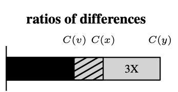
In practical settings, one is concerned with the meaningful statements that can be made about the values of the SCF \( C\) evaluated for different outcomes. For example, by selecting \( z=w=v\) in (1), the ratios-of-differences takes the form
which has an immediate interpretation: going from allocation \( v\) to allocation \( x\) is \( t\) times better/worse than going from allocation \( v\) to allocation \( y\) .
It should not be surprising that other operations on the SCF \( C\) are not generally permissible: \( C\) is a cardinal representation of the order imposed by the SCFL \( \mathfrak F\) . Therefore, additional measures, such as setting a fixed reference point or a fixed scale, are needed to make other operations (e.g., absolute differences or ratios) meaningful.
4 Examples
In this section, we illustrate how the methodology proposed in this paper is applicable to engineering problems comprising multiple agents competing for a limited resource. We considered two timely domains: water allocation and traffic control. We illustrate how a designer can decide the appropriate interpersonal comparability level, considering the available information and societal or political perceptions, and select an appropriate social cost function.
4.1 Water allocation
Agricultural irrigation accounts for 70% of global freshwater use already, and projections are that irrigation-based food production will need to grow another 50% by 2050 due to climate change in combination with population growth [44]. As groundwater reservoirs deplete [45], water will need to be used more efficiently and prudently to avoid resource collapse [46], and allocation/priority rules are needed to avoid a “tragedy of the commons” [47]. Recent works have explored advanced control techniques for water allocation [48, 49, 50, 51].
Comparability
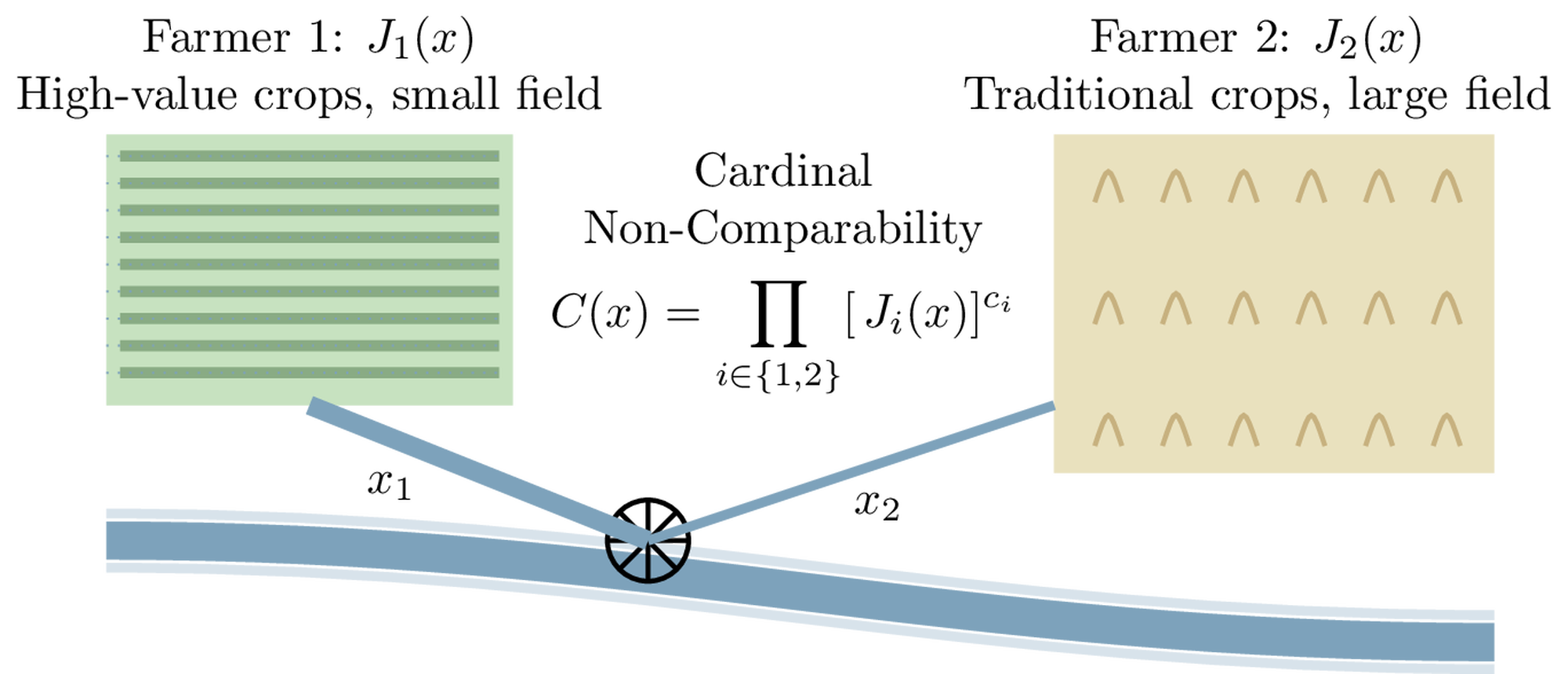
In irrigation systems, the value a farmer draws from a certain amount of allocated water is difficult to quantify, especially as agricultural farmland and resulting needs are heterogeneous due to crops requiring different amounts of water per hectare and across seasons, with all of it being precipitation dependent [44, 46]. Thus, one can only conclude that farmers generally experience increased benefits with higher water allocations, though comparing it across heterogeneous farmers is not appropriate [52] (Figure 4). As stated in [53], regulators are interested in designing schemes that robustly satisfy social welfare and justice criteria despite this unmeasurable heterogeneity. These considerations, in the context of comparability, correspond to Cardinal Non Comparability of farmers’ costs.
Choice of SCF
Under CNC, the appropriate social welfare function is the Nash Social Welfare. For the purpose of water allocation, farmers usually own water rights or water shares to cover the size of their land and account for the crop they are growing. In such a setting, the axiom of Anonymity (A) is not appropriate as the allocation must consider farmers’ different access rights to water. Thus, different exponents \( c_i\) are allowed and appropriate in the SCF.
Implications of the choice of SCF
Consider a simplified example where every farmer \( i\) has water rights \( c_i\) and receives a proportion \( x^{(i)}\) of the total available water \( \bar X\) . We assume farmers have an upfront cost every season \( J_i(x_0)\) and draw marginal utility from an increased water allocation \( q_i x^{(i)}\) , so that the cost of farmer \( i\) is given by \( J_i(x) = J_i(x_0) - q_i x^{(i)}\) . The resulting SCF problem becomes
(2)
An interesting case arises when we solve for the optimal social outcome independent of the upfront costs (which the farmers may not disclose); thus, \( J_i(x_0)\) (no water, i.e., \( x_0^{(i)} = 0\forall i\) ) acts as a natural worst-case benchmark, corresponding to a planner’s choice not to consider upfront expenses. This is reasonable when only water rights should influence the allocation rule. Thus, the farmers themselves need to trade off their costs and marginal benefits with every water share they buy. This approach considers the practical difficulty for a social planner to verify and measure farmers’ true expenses or worst-case states.
In such a case, the SCF becomes \( -\prod_{i} \left[\,q_i x^{(i)}\right]^{c_i}\) . The solution of (2) then satisfies proportional fairness [54], which coincides with the proportional allocation
(see derivation in the appendix of [55]).
Proportional allocation is a commonly used allocation procedure implemented in constituencies worldwide [56, 57, 52, 58]. Thus, using social choice theory arguments and analyzing the underlying comparability notion we were able to give a different perspective on the commonly used proportional allocation rule in water irrigation systems.
4.2 Traffic Control
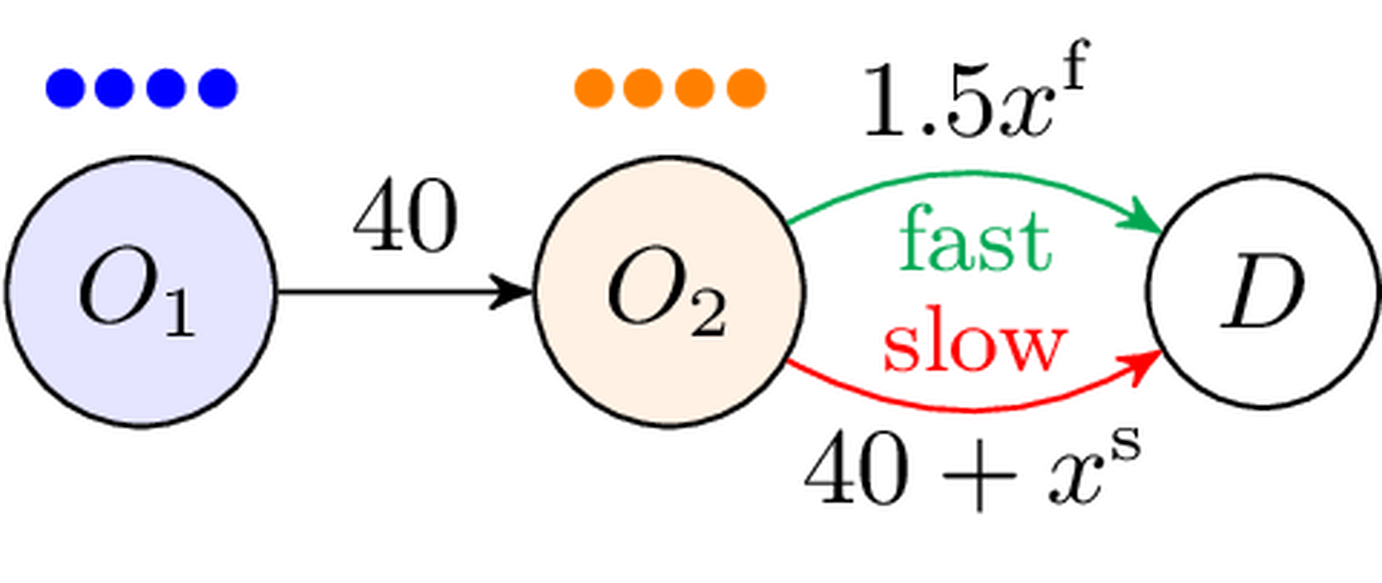
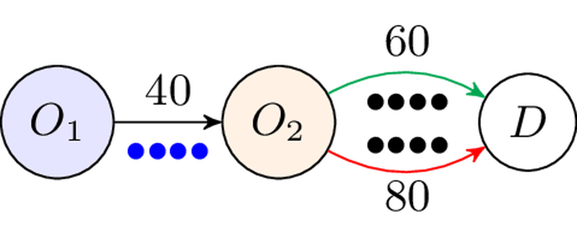
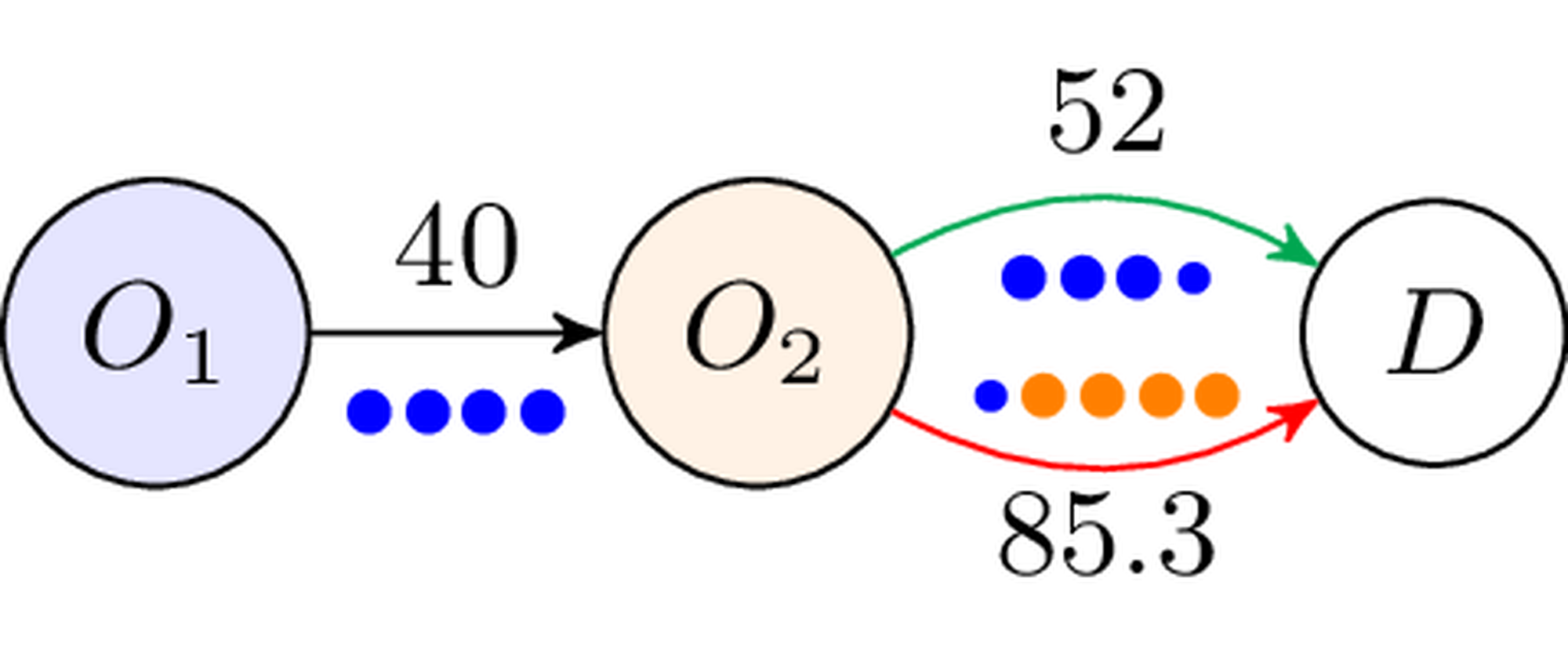
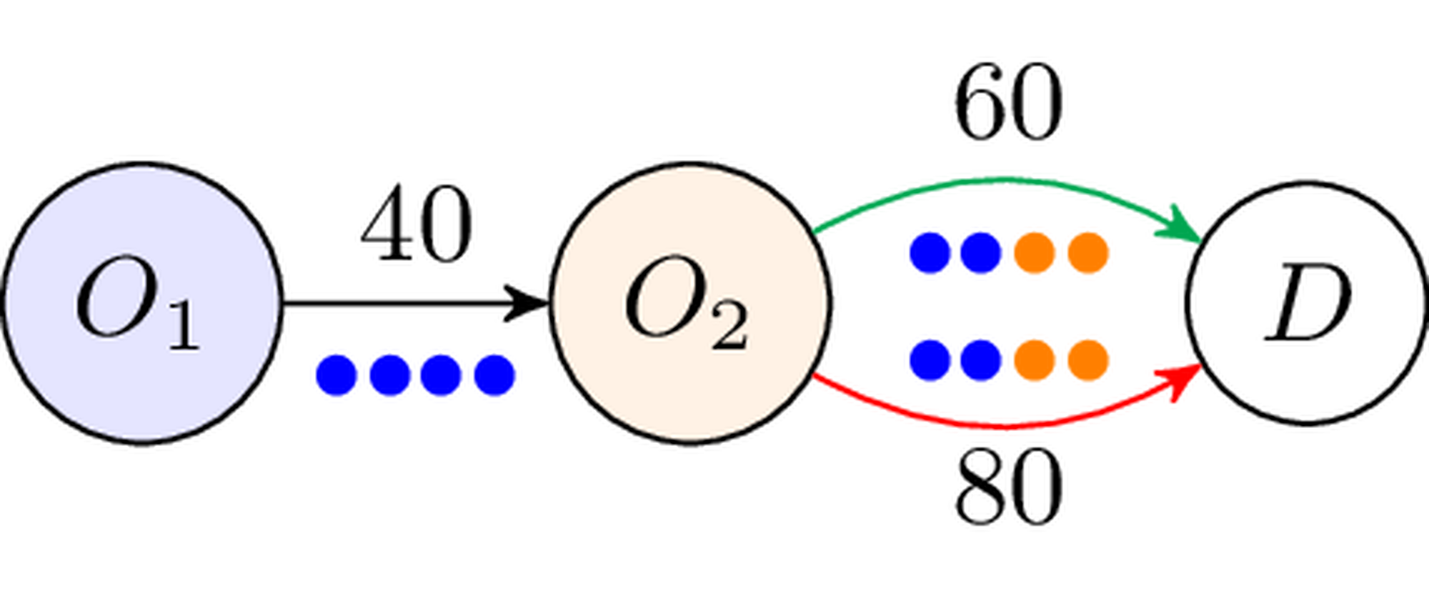
Fig. 5 shows an example of the commonly studied traffic routing problem [14, 15, 16, 17] with \( 40\) long-distance commuters travelling from \( O_1\) through \( O_2\) to \( D\) , and \( 40\) short-distance commuters travelling from \( O_2\) to \( D\) only. The link delays are as shown in Fig. 6. We next discuss whether travel delay costs of both commuter types can be compared and illustrate the consequences of different comparability assumptions.
Comparability
The prevalence of the sum of costs as SCF in the literature suggests that either (CUC) or (CFC) is implicitly assumed. (CUC) is often assumed in conjunction with tolling solutions [59], in which the unit of comparison is the monetary value of time [10], and the commuters’ dispensable incomes, i.e., the affine offsets \( b_i\) , are not considered in the cost functions. Works that instead explicitly account for income differences[24] can be classified under (CFC). (CFC) is also natural when considering the travel delays themselves as costs (and not how they convert to money), with the justification that everyone has 24 hours in a day.
One could instead assume that travel delays are non-comparable (CNC), justified as follows. The commuter heterogeneity is attributed to non-comparable trade-offs, e.g., long-distance commuters prioritize large housing over short commutes, and vice versa for short-distance commuters.
Choice of SCF
In addition to basic axioms (P), (IIA), Anonymity (A) is desired if commuters are to have equal access rights to roads. Therefore, under (CUC) the only appropriate SCF is \( \sum_i J_i\) , while a larger family of SCFs is permissible under (CFC) (see Table 1). To balance a trade-off between total delays and delays of the worst off, one can choose SCF \( \sum_i J_i + \gamma \max J_i\) . In our example, \( \gamma\) essentially dictates to what extent long-distance commuters should be compensated in \( O_2 \rightarrow D\) for their additional delay in \( O_1 \rightarrow O_2\) . Under (CNC), since travel delay costs are nonnegative, one must resort to Partial Independence (PI), and choose a suitable reference outcome \( x_0\) . A natural choice of \( x_0\) is the non-controlled traffic equilibrium, since it represents the status quo or disagreement point if negotiations to adopt new control policies fail, and is commonly adopted in transportation to certify that policies are Pareto improving [60, 27]. This leads to SCF \( \prod_i \left(J_i^\textup{eq} - J_i\right)\) , with \( J_i^\textup{eq}\) denoting the equilibrium delay to commuter \( i\) .
Implications of the choice of SCF
The SCF can be used in an optimization formulation to determine the socially optimal traffic outcome. Figs. 7–9 illustrate the results in our example network, indicating the optimal link delays and associated allocations of long-distance (blue) and short-distance (orange) commuters . Notice that under (CUC), it does not matter which commuter uses the fast/slow link (indicated black in Fig. 7). While these different allocations may appear intuitively more or less fair or efficient, we emphasize that the appropriate notion of ‘fairness and efficiency’ is underpinned by the assumed and justifiable level of comparability.
5 Conclusions
Much of applied control work has implicitly been performed with the interests of the population in mind and based on “welfarist” principles as we laid out in this document. This work aims to provide guidance for making the foundations of the use of social cost functions explicit and, thus, to enable control theorists to express and defend their objectives based on the limits/possibilities of interpersonal comparability in various contexts and applications. In some cases, some social cost functions have to be ruled out, while many functions are permissible in other situations, and our theory thus may restrict or make explicit the range of control objectives that an engineer may pursue. The theoretical and empirical foundations that render different social cost functions preferable (e.g., the efficiency-equity tradeoff in the choice of a SCF under CFC) deserve further investigation.
A Nash welfare and proportional allocation
Proportional allocation rules (and their relation to proportional fairness and to Nash welfare) have been derived and discussed originally for networking applications, see [54]. In the following, we give a short proof for the special case that is relevant for the water allocation example presented in Section 4.1.
Consider the problem of allocating \( \bar X\) water resources with each agent having cost \( J_i(x) = -q_i x^{(i)}\) and water rights \( c_i\) . To derive the optimal strategy under Nash social welfare we begin by restating the Nash welfare function as a SCF
under which the water allocation problem becomes
We know that the positive allocation constraint is not active and consequently only dualize the coupling constraint. The corresponding Lagrangian is \( L(x,\lambda) = -\sum c_i \log(q_ix^{(i)}) + \lambda (\sum x^{(i)} - \bar X) \) and by the principle of optimality we have:
thus \( x^{(i)*} = \frac{c_i}{\lambda}\) , further primal feasibility yields
and, consequently, the optimal allocation strategy corresponds to a proportional allocation
where each agent receives a fraction of the total water proportional to their water rights.
References
[1] A. M. Annaswamy, K. H. Johansson, and G. J. Pappas, Eds., Control for Societal-scale Challenges: Road Map 2030. 1em plus 0.5em minus 0.4em IEEE Control Systems Society, 2023. [Online]. Available: https://ieeecss.org/control-societal-scale-challenges-roadmap-2030
[2] I. Caragiannis, D. Kurokawa, H. Moulin, A. D. Procaccia, N. Shah, and J. Wang, “The unreasonable fairness of maximum Nash welfare,'' in ACM EC, 2019.
[3] S. Ramezani and U. Endriss, “Nash social welfare in multiagent resource allocation,'' in International Workshop on Agent-Mediated Electronic Commerce. 1em plus 0.5em minus 0.4em Springer, 2009, pp. 117–131.
[4] B. Radunović and J.-Y. Le Boudec, “A unified framework for max-min and min-max fairness with applications,'' IEEE/ACM Trans. on Networking, vol. 15, no. 5, pp. 1073–1083, 2007.
[5] D. Bertsimas, V. F. Farias, and N. Trichakis, “The price of fairness,'' Operations Research, vol. 59, no. 1, pp. 17–31, 2011.
[6] V. X. Chen and J. N. Hooker, “A guide to formulating fairness in an optimization model,'' Annals of Operations Research, vol. 326, pp. 581–619, Apr. 2023.
[7] M. Maciejewski, J. Bischoff, and K. Nagel, “An assignment-based approach to efficient real-time city-scale taxi dispatching,'' IEEE Trans. Intelligent Systems, vol. 31, no. 1, pp. 68–77, 2016.
[8] X. Luan, F. Corman, and L. Meng, “Non-discriminatory train dispatching in a rail transport market with multiple competing and collaborative train operating companies,'' Transportation Research Part C: Emerging Technologies, vol. 80, pp. 148–174, 2017.
[9] T. Sousa, T. Soares, P. Pinson, F. Moret, T. Baroche, and E. Sorin, “Peer-to-peer and community-based markets: A comprehensive review,'' Renewable and Sustainable Energy Reviews, vol. 104, pp. 367–378, 2019.
[10] L. Zamparini and A. Reggiani, “Meta-analysis and the value of travel time savings: a transatlantic perspective in passenger transport,'' Networks and Spatial Economics, vol. 7, no. 4, pp. 377–396, 2007.
[11] Y. Liu, Z. Liu, and K. Savla, “Adaptive pricing for routing game identification: Theory & experiment,'' IFAC-PapersOnLine, vol. 58, no. 30, pp. 13–18, 2024.
[12] D. Muthirayan, D. Kalathil, K. Poolla, and P. Varaiya, “Mechanism design for demand response programs,'' IEEE Trans. on Smart Grid, vol. 11, no. 1, pp. 61–73, 2019.
[13] F. Munoz, A. Nayak, and S. Lee, Engineering Applications of Social Welfare Functions. 1em plus 0.5em minus 0.4em Springer International Publishing, 2023, vol. 13.
[14] R. Chandan, D. Paccagnan, and J. R. Marden, “Methodologies for quantifying and optimizing the price of anarchy,'' IEEE Trans. on Automatic Control, vol. 69, pp. 7742–7757, Nov. 2024.
[15] J. Zhang, S. Pourazarm, C. G. Cassandras, and I. C. Paschalidis, “The price of anarchy in transportation networks: Data-driven evaluation and reduction strategies,'' Proceedings of the IEEE, vol. 106, pp. 538–553, Apr. 2018.
[16] G. Piliouras, E. Nikolova, and J. S. Shamma, “Risk sensitivity of price of anarchy under uncertainty,'' ACM Trans. on Economics and Computation, vol. 5, pp. 1–27, Feb. 2017.
[17] X. Wang, N. Xiao, L. Xie, E. Frazzoli, and D. Rus, “Analysis of price of total anarchy in congestion games via smoothness arguments,'' IEEE Trans. on Control of Network Systems, vol. 4, pp. 876–885, Dec. 2017.
[18] C. Hill and P. N. Brown, “The tradeoff between altruism and anarchy in transportation networks,'' in IEEE ITSC, 2023.
[19] A. Jadbabaie, A. Ozdaglar, and M. Zargham, “A distributed Newton method for network optimization,'' in IEEE CDC, 2009.
[20] A. Menon and J. S. Baras, “Collaborative extremum seeking for welfare optimization,'' in IEEE CDC, 2014.
[21] J. J. Romvary, G. Ferro, R. Haider, and A. M. Annaswamy, “A proximal atomic coordination algorithm for distributed optimization,'' IEEE Trans. on Automatic Control, vol. 67, no. 2, pp. 646–661, 2021.
[22] F. Farhadi, S. J. Golestani, and D. Teneketzis, “A surrogate optimization-based mechanism for resource allocation and routing in networks with strategic agents,'' IEEE Trans. on Automatic Control, vol. 64, pp. 464–479, Feb. 2019.
[23] R. Maheswaran and T. Basar, “Social welfare of selfish agents: motivating efficiency for divisible resources,'' in IEEE CDC, 2004.
[24] D. Jalota, K. Solovey, K. Gopalakrishnan, S. Zoepf, H. Balakrishnan, and M. Pavone, “When efficiency meets equity in congestion pricing and revenue refunding schemes,'' in 1st ACM Conf. on Equity and Access in Algorithms, Mechanisms, and Optimization, 2021.
[25] E. Villa, V. Breschi, and M. Tanelli, “Fair-MPC: A framework for just decision-making,'' IEEE Transactions on Automatic Control, 2025.
[26] H. Bang, A. Dave, F. N. Tzortzoglou, and A. A. Malikopoulos, “A mobility equity metric for multi-modal intelligent transportation systems,'' IFAC-PapersOnLine, vol. 58, no. 10, pp. 114–119, 2024.
[27] E. Elokda, C. Cenedese, K. Zhang, A. Censi, J. Lygeros, E. Frazzoli, and F. Dörfler, “Carma: Fair and efficient bottleneck congestion management via nontradable karma credits,'' Transportation Science, 2024.
[28] P. P. Khargonekar, T. Samad, S. Amin, A. Chakrabortty, F. Dabbene, A. Das, M. Fujita, M. Garcia-Sanz, D. F. Gayme, M. Ilić et al., “Climate change mitigation, adaptation, and resilience: Challenges and opportunities for the control systems community,'' IEEE Control Systems Magazine, vol. 44, no. 3, pp. 33–51, 2024.
[29] J. R. Marden and A. Wierman, “Distributed welfare games,'' Operations Research, vol. 61, pp. 155–168, Feb. 2013.
[30] E. Jensen and J. R. Marden, “Optimal utility design in convex distributed welfare games,'' in ACC, 2018.
[31] J. R. Marden and T. Roughgarden, “Generalized efficiency bounds in distributed resource allocation,'' IEEE Trans. on Automatic Control, vol. 59, pp. 571–584, Mar. 2014.
[32] C. d'Aspremont and L. Gevers, “Equity and the informational basis of collective choice,'' The Review of Economic Studies, vol. 44, no. 2, pp. 199–209, 1977.
[33] K. W. S. Roberts, “Interpersonal comparability and social choice theory,'' The Review of Economic Studies, vol. 47, no. 2, pp. 421–439, 1980.
[34] C. d'Aspremont and L. Gevers, “Social welfare functionals and interpersonal comparability,'' in Handbook of Social Choice and Welfare, K. J. Arrow, A. K. Sen, and K. Suzumura, Eds. 1em plus 0.5em minus 0.4em Elsevier, 2002, vol. 1, ch. 10, pp. 459–541.
[35] A. Sen, “Utilitarianism and welfarism,'' Journal of Philosophy, vol. 76, no. 9, pp. 463–489, 1979.
[36] J. Bentham, An Introduction to the Principles of Morals and Legislation. 1em plus 0.5em minus 0.4em London: T. Payne and Son, 1789.
[37] J. C. Harsanyi, “Cardinal welfare, individualistic ethics, and interpersonal comparisons of utility,'' Journal of Political Economy, vol. 63, no. 4, pp. 309–321, 1955.
[38] J. Rawls, A Theory of Justice. 1em plus 0.5em minus 0.4em Cambridge, MA: Belknap Press of Harvard University Press, 1971.
[39] J. F. Nash, “The bargaining problem,'' Econometrica, vol. 18, no. 2, pp. 155–162, 1950.
[40] M. Kaneko and K. Nakamura, “The Nash social welfare function,'' Econometrica, vol. 47, no. 2, pp. 423–435, 1979.
[41] A. Sen, “Interpersonal aggregation and partial comparability,'' Econometrica: Journal of the Econometric Society, pp. 393–409, 1970.
[42] P. J. Hammond, “Roberts’ weak welfarism theorem: a minor correction,'' Social Choice and Welfare, vol. 60, pp. 121–134, 2023.
[43] H. Kraft and C. Procesi, A Primer of Classical Invariant Theory: Preliminary Version. 1em plus 0.5em minus 0.4em Éditeur inconnu, 1996, 126 pages.
[44] E. Bwambale, F. K. Abagale, and G. K. Anornu, “Smart irrigation monitoring and control strategies for improving water use efficiency in precision agriculture: A review,'' Agricultural Water Management, vol. 260, p. 107324, Feb. 2022.
[45] L. E. Condon, S. Kollet, M. F. P. Bierkens, G. E. Fogg, R. M. Maxwell, M. C. Hill, H. H. Fransen, A. Verhoef, A. F. Van Loon, M. Sulis, and C. Abesser, “Global groundwater modeling and monitoring: Opportunities and challenges,'' Water Resources Research, vol. 57, no. 12, Dec. 2021.
[46] M. Li, W. Xu, and M. W. Rosegrant, “Irrigation, risk aversion, and water right priority under water supply uncertainty,'' Water Resources Research, vol. 53, no. 9, pp. 7885–7903, Sep. 2017.
[47] O. Olorunfemi. (2023, September) How solar water pumps are changing smallholder farming in Africa. Yale Environment 360. [Online]. Available: https://e360.yale.edu/features/solar-water-pumps-groundwater-crops
[48] R. R. Negenborn, P.-J. van Overloop, T. Keviczky, and B. De Schutter, “Distributed model predictive control of irrigation canals,'' Networks and Heterogeneous Media, vol. 4, no. 2, pp. 359–380, Jun. 2009.
[49] A. Castelletti, A. Ficchì, A. Cominola, P. Segovia, M. Giuliani, W. Wu, S. Lucia, C. Ocampo-Martinez, B. De Schutter, and J. M. Maestre, “Model predictive control of water resources systems: A review and research agenda,'' Annual Reviews in Control, vol. 55, pp. 442–465, 2023.
[50] J. Val Ledesma, R. Wisniewski, C. S. Kallesøe, and A. Tsouvalas, “Water age control for water distribution networks via safe reinforcement learning,'' IEEE Trans. on Control Systems Technology, vol. 32, no. 6, pp. 2332–2343, Nov. 2024.
[51] Y. Wang, E. Weyer, C. Manzie, A. R. Simpson, and L. Blinco, “Stochastic co-design of storage and control for water distribution systems,'' IEEE Trans. on Control Systems Technology, vol. 33, no. 1, pp. 274–287, Jan. 2025.
[52] J. A. Gómez-Limón, C. Gutiérrez-Martín, and N. M. Montilla-López, “Agricultural water allocation under cyclical scarcity: The role of priority water rights,'' Water, vol. 12, no. 6, p. 1835, Jun. 2020.
[53] K. Madani and A. Dinar, “Exogenous regulatory institutions for sustainable common pool resource management: Application to groundwater,'' Water Resources and Economics, vol. 2–3, pp. 57–76, 2013.
[54] F. P. Kelly, A. K. Maulloo, and D. K. H. Tan, “Rate control for communication networks: shadow prices, proportional fairness and stability,'' Journal of the Operational Research Society, vol. 49, pp. 237–252, Mar. 1998.
[55] I. Shilov, E. Elokda, S. Hall, H. H. Nax, and S. Bolognani, “Welfare and cost aggregation for multi-agent control: When to choose which social cost function, and why?'' arXiv preprint, 2025.
[56] E. Ostrom, R. Gardner, and J. Walker, Rules, Games, and Common-Pool Resources. 1em plus 0.5em minus 0.4em University of Michigan Press, 1994.
[57] M. C. Roa-García, “Equity, efficiency and sustainability in water allocation in the Andes: Trade-offs in a full world,'' Water Alternatives, vol. 7, pp. 298–319, 2014.
[58] M. W. Rosegrant and H. P. Binswanger, “Markets in tradable water rights: Potential for efficiency gains in developing country water resource allocation,'' World Development, vol. 22, no. 11, pp. 1613–1625, Nov. 1994.
[59] H. Yang and H.-J. Huang, “Principle of marginal-cost pricing: how does it work in a general road network?'' Transportation Research Part A: Policy and Practice, vol. 32, no. 1, pp. 45–54, 1998.
[60] C. F. Daganzo and R. C. Garcia, “A Pareto improving strategy for the time-dependent morning commute problem,'' Transportation Science, vol. 34, no. 3, pp. 303–311, 2000.