
Documents Live, a web authoring and publishing system
If you see this, something is wrong
Table of contents
First published on Wednesday, Jul 16, 2025 and last modified on Wednesday, Jul 16, 2025 by François Chaplais.
Abstract
Discovering governing equations that describe complex chaotic systems remains a fundamental challenge in physics and neuroscience. Here, we introduce a method, the PEM-UDE, that combines the prediction-error method with universal differential equations to extract interpretable mathematical expressions from chaotic dynamical systems, even with limited or noisy observations. This approach succeeds where traditional techniques fail by smoothing optimization landscapes and removing the chaotic properties during the fitting process without distorting optimal parameters. We demonstrate its efficacy by recovering hidden states in the Rössler system and reconstructing dynamics from noise-corrupted electrical circuit data, where the correct functional form of the dynamics are recovered even when one of the observed time series is corrupted by noise 5x the magnitude of the true signal. We showcase that this method with prior knowledge embeddings is able to recover the correct dynamics where direct symbolic regression methods, such as STLSQ, fail with the given amount of data and noise. Importantly, when applied to neural populations, our method derives novel governing equations that respect biological constraints such as network sparsity – a constraint necessary for cortical information processing yet not captured in next-generation neural mass models – while preserving microscale neuronal parameters. These equations predict an emergent relationship between connection density and both oscillation frequency and synchrony in neural circuits. We validate these predictions using three intracranial electrode recording datasets from the medial entorhinal cortex, prefrontal cortex, and orbitofrontal cortex. Our work provides a pathway to develop mechanistic, multi-scale brain models that generalize across diverse neural architectures, bridging the gap between single-neuron dynamics and macroscale brain activity.
1 Introduction
Discovering the equations that govern complex systems has been the goal of dynamics for much of the past century and frequently requires both an expert knowledge of the domain of application and a fair understanding of statistical mechanics to achieve [1, 2, 3, 4]. When successful, this approach has led to significant advancements in our ability to model and predict the behavior of complex systems in applications ranging from climate models [5, 6] to chemical reactions [7, 8] to human social interactions [9]. Recent advances in complex systems theory rely on automated approaches to equation discovery, which have emerged to assist the normally expert-driven process of describing data with systems of differential equations [10, 11, 12, 13]. Symbolic regression techniques, including sparse identification methods (SINDy; [10]) and genetic algorithm approaches [14], have been developed to fit equations directly from data. Although promising, these approaches are limited by their difficulties fitting noisy data [15]. More recently, Universal Differential Equations (UDEs) have emerged as a powerful approach that combines the strengths of machine learning with traditional scientific computing techniques [16]. UDEs incorporate artificial neural networks within differential equation frameworks to learn unknown dynamics directly from data. This approach relies on training a universal approximator under two constraints: imposing a known functional form on the dynamics before learning additional unknown terms [16], and imposing structural constraints on the learning process itself [17].
While useful, these approaches struggle when fitting chaotic systems, which are ubiquitous in neuroscience and other biological contexts [18, 19, 20, 21]. Even simple physical systems can exhibit complex, chaotic solutions when certain parameters are brought past a bifurcation point [22]. Neural dynamics, in particular, often display characteristics of chaotic oscillators [20, 23]. The presence of chaos introduces numerical problems in the fitting, as the trajectory of a chaotic system is not well-defined beyond a Lyapunov time. Formally, any numerical ODE solver introduces truncation error in each step and, due to sensitive dependence on inputs, that ODE solver output will have an \( O(1)\) error in the produced trajectory shortly after a Lyapunov time. The only guarantee that the numerical simulation gives a meaningful trajectory is provided by the shadowing lemma, which states that there exists an epsilon ball around the initial condition in which the numerical solver’s trajectory matches the trajectory of one of the other potential initial conditions within the epsilon ball (a statement of density of solutions around the attractor) [24]. The shadowing lemma introduces two crucial factors that make it a particularly challenging problem to learn. The divergent nature of chaotic trajectories creates fundamental instability in all sensitivity analysis methods used to compute gradients. This instability means that standard automatic differentiation through solvers produces inaccurate derivative estimates unless specialized modifications are applied [25, 26, 27, 28, 29]. As a consequence, the standard method for calibration of trajectories, i.e. fitting a loss function defined by numerical solutions of the ODE solver, is not a convergent algorithm in the context of chaotic systems. Additionally, noisy observational data can create a loss function that cannot distinguish between nearby trajectories during training, leading to inaccuracies in the fit dynamics [24]. In other words, with exponential dependence of the solution on initial parameters, infinitesimal changes to the data may land the data point exponentially further along the time series trajectory. Because of these properties, the long-term time series of a chaotic system can only be interpreted probabilistically, based on statistical or ergodic properties [30, 31, 32]. This makes the traditional techniques of fitting a time series via the L2 norm simply ill-defined in these chaotic contexts. Finally, in real-world models, we additionally only have partial observability, which makes parameter fitting for any dynamical system challenging. This is particularly true in neuroscience, where neural interactions form complex systems operating across multiple scales—from molecular processes like neurotransmitter activity to brain-wide electric fields that can be observed on EEG [33, 19, 34].
Aside from the complexity inherent in describing these multi-scale interactions, the dynamics of the brain are often poised near “critical points” that allow for adaptive switching between different dynamic states depending on task requirements, metabolic resources available, and overall health of the neural circuits [35, 36, 37]. While there is an advantage to flexibility and information processing by being located at these critical points, this means that neural dynamics are intrinsically sensitive to small perturbations [38, 20]. Traditional approaches to modeling neuron populations, termed neural mass models, focused on capturing specific macroscale properties without a systematic approach to accounting for microscale biophysical parameters (e.g., ion channel conductance) [39, 40, 41]. More recently, next-generation neural mass models have been shown to provide an analytical expression for population-level activity that preserves the microscale detail present in individual neurons while also capturing emergent macroscale properties (e.g., time-varying synchrony) [42, 43, 44]. These analytical approaches typically rely on the Ott-Antonsen ansatz [45] to avoid a Fokker-Planck derivation of the mean-field dynamics [46, 47]. An important caveat of these derivations is that while they capture many desirable multi-scale dynamics, they rely on non-biophysical assumptions (e.g., all-to-all connectivity between neurons [42], current conservation throughout the system [47]). Although neuron-scale simulations that violate these assumptions are possible, it is difficult or impossible to analytically account for these violations in new derivations of neural masses, thereby limiting their applications to full-scale brain models.
The fundamental disconnect between the underlying neurobiology and the assumption of fully-connected networks that underlies these derivations presents both a challenge and an opportunity. While this assumption is approximately true for deep and subcortical structures [43], it is far from physiological in the cortex, where only 1-5% connectivity is the norm [48]. This is also not an evolutionary afterthought or accident, as there are converging streams of evidence that the sparse, structured connectivity patterns exhibited in the cortex are essential for structured information flow that gives rise to higher cognitive processes [49, 50]. Accurately accounting for sparsity in equations that capture population activity is therefore a necessity in developing accurate models of the brain.
To overcome these limitations, we present a novel method for training UDEs to fit chaotic system dynamics. We apply this method to derive novel next-generation neural mass models that generalize from subcortical to cortical dynamics. We begin by describing the procedure, which leverages the prediction-error method (PEM) [17, 51] to assist in training the UDEs on chaotic system data, and then derives a symbolic form of the learned expression from the UDE to generalize the dynamics. We demonstrate the ability of this approach to learn unknown states in a chaotic system, showing that it can accurately recover a hidden state in the Rössler system that traditional UDE approaches cannot and that it does so by removing the sensitive dependence on parameter choices from the system. We then demonstrate that our approach learns the dynamics of a chaotic electrical circuit even under incomplete observation of states, where a dimension of the observed data is corrupted by noise 5x the original signal. Notably, we showcase that the PEM-UDE approach is more data-efficient than pure symbolic regression by demonstrating that sequential thresholding least squares (STLSQ) is unable to recover the correct dynamic system under these conditions. Finally, we demonstrate the system’s ability to learn the dynamics of a neural mass model directly from the firing rate and voltage of a network of spiking neurons, showing that it can successfully learn the mean-field dynamics from data that are typically the only states observable experimentally. Our approach demonstrates that the symbolic form we have developed generalizes across different brain regions more effectively than traditional neural mass models. Our modeling directly reveals how varying connectivity structures throughout the brain produce distinct rhythmic patterns in different regions.
2 Results
2.1 Formal description of approach
2.1.1 Overview
We provide a formal definition of the combined PEM-UDE/symbolic regression method to motivate our approach and demonstrate the method’s novelty. We explore arguments for why our method works where traditional systems fail to learn chaotic dynamics. Implementation details are given in the Methods section and accompanying code. The associated repository includes a demonstration using toy data that runs efficiently on standard computers for interested readers.
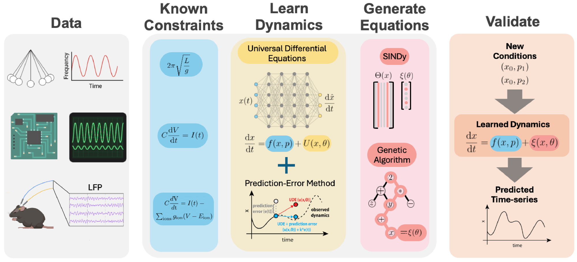
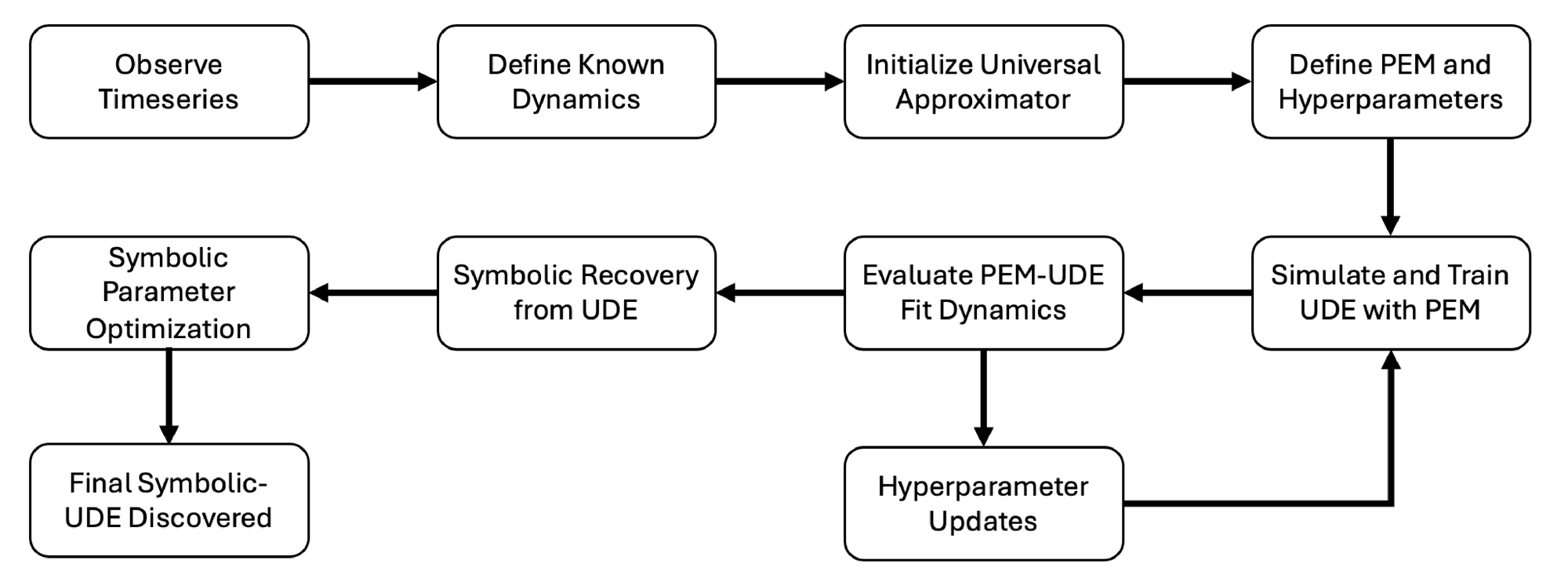
A graphical overview of the approach is provided in Fig. 1. We begin with observations of a physical or biological system that result in a dataset of related time series. Ideally, we would like to have a complete system of differential equations that describes the dynamics of the system under observation and makes accurate predictions of future dynamics. Based upon these observations and previous work on similar systems, we can create an initial guess of a description of the dynamics, leveraging prior information from physical systems to structure the first approximation of the system’s behavior [16]. We then set up a UDE system to learn the unknown dynamics directly from the observed data. Traditional methods for training UDEs struggle to accurately fit chaotic systems, as shown in the results. To address this limitation, we developed a novel training approach that integrates PEM dynamics with the UDE during simulations, enabling accurate learning from the data. Once training is complete, we extract a symbolic representation of the dynamics from the UDE network using either sparse linear solver based symbolic regression techniques (STLSQ) or with evolutionary algorithm based symbolic regression methods [14], depending on the specific context and data availability. This symbolic description allows us to both predict future time series and make analytical observations about the underlying dynamics.
2.1.2 UDE approach
Following prior work [16], a universal differential equation (UDE) with an additive correction of a general process \( \mathbf{x}(t)\) with some observable state \( \mathbf{y}(t)\) is given by
(1.a)
Here we use bold variables to denote vectors. \( f_p\) are the known (or assumed) dynamics of the system with parameters \( p\) , \( \mathbf{x}_{p,\theta}(t; \mathbf{x}_0)\) denotes the solution of those dynamics with initial conditions \( \mathbf{x}_0\) at parameter values \( p\) and \( \theta\) , \( \mathbf{u}(t)\) is an external stimulus, \( h_q(\mathbf{x}_{p,\theta}(t; \mathbf{x}_0), t)\) is the observation function parameterized by \( q\) which can explicitly depend on time (for instance, due to some noise processes or the influence of the external stimulus on the observation etc.), and \( NN_\theta(\mathbf{x})\) is the universal approximator network trained to learn the unknown dynamics of the system based on its parameters \( \theta\) . Lastly, note that for notational simplicity we drop the parameter dependence of the observation \( \mathbf{y}_\theta(t)\) on parameters \( p\) and \( q\) and initial conditions \( \mathbf{x}_0\) , but keep the network parameters \( \theta\) since we want to optimize those while keeping the rest fixed. While this work focuses on systems of ordinary differential equations, it is not limited to these scenarios, and can be extended to stochastic and delayed differential equation systems as well, as has been done in previous work using UDEs [16]. For some observed dataset \( \{\hat{\mathbf{y}}_i\}_{i=1, \dots, N}\) , training the UDE \( NN_\theta\) will use a cost function \( C(\theta)\) that minimizes the error at every observed time point \( t_i\) such that
(2)
where \( \mathbf{y}_\theta(t_i)\) is the observed solution of the ODE with neural network weights \( \theta\) at the measurement times \( t_i\) . In all equations that rely on observational data, we define any observed data for \( \mathbf{x}\) to be denoted as \( \hat{\mathbf{x}}\) . Although we chose \( C(\theta)\) to be the mean squared error in this work, many other cost functions are appropriate for different scenarios, depending on how measurement noise affects the measured signal. We then use the prediction-error method to train UDEs on this loss function for chaotic systems.
2.1.3 PEM approach
The prediction-error method (PEM) is a standard optimization technique in fitting parameters of dynamical systems to observational data [17, 52]. Similarly to Eq. (1), we consider a general process \( \mathbf{x}(t)\) that gives rise to some observable state \( \mathbf{y}(t)\) with some measurement noise \( \mathbf{e}(t)\)
(3.a)
In this statement, \( \mathbf{x}\) is the state of a time-varying system with parameters \( p\) that we wish to fit. The observed state \( \mathbf{y}\) is defined by a measurement function \( m\) of the process \( \mathbf{x}(t)\) , parameterized by \( q\) , and a measurement error \( \mathbf{e}(t)\) . Here, we assume that there is a one-to-one mapping of \( \mathbf{x}\) to \( \mathbf{y}\) (i.e., there are no terms in \( \mathbf{y}\) that depend on multiple elements of \( \mathbf{x}\) ). For a more general discussion of the conditions under which PEM can be applied, see [17, 52]. For example, \( m_{q,i}\) is not limited to being a linear function of \( x_i\) , but can also perform a convolution or incorporate delays [52]. In all of our examples, a few components of \( m_{q,i}\) are zero, indicating that these components, \( y_{p,i}\) , are not observed. The estimation error \( \epsilon\) is weighted by a function \( K(t, \beta)\) and is added at each time step to the original dynamics \( \mathbf{x}(t)\) to create an adjusted estimate \( \tilde{\mathbf{x}}(t)\) and observations \( \tilde{\mathbf{y}}(t)\) such that
(4.a)
where, as defined above, \( \hat{\mathbf{y}}(t)\) is the observed data, interpolated to whatever step is needed by the solver. This error gain factor \( K(t, \beta)\) can take on different forms. In this work, we set \( K(t, \beta)=K\) , thereby employing the simplest possible form of what previous work has called the parameterized observer [52]. If there is strong reason to suspect that the quality of the observations varies over time (e.g. significantly increased noise present at certain time intervals), then including this information in a time-varying \( K(t, \beta)\) for instance by expanding the equations (4) to resemble an extended Kalman filter (where \( K(t, \beta)\) is the Kalman gain), could provide better performance when fitting. However, we note that previous work has shown that the parameterized observer outperforms the extended Kalman filter in practice, as tuning the hyperparameter over time is difficult [52]. Although for notational simplification we will use \( K\) in the remaining sections, this is done without loss of generality, as implementing an extended Kalman filter can easily be done if there is a data-driven reason to require it.
The PEM approach then seeks to find the optimal set of parameters \( \hat p\) such that
(5)
which resembles the same objective function as defined above for the UDE optimization. As with Eq. 2, we choose here the mean squared error, but the PEM approach will work with any reasonable distance function \( \epsilon_p\) .
2.1.4 Combining PEM-UDE into single method
Our approach in this paper trains UDEs to learn chaotic systems using the PEM to tame the sensitivity to parameter choices to a sufficient degree that the dynamics can be accurately recovered. Formally, we express this system as a combination of Eq. (1) and Eq. (4) such that
(6.a)
where, as defined above, \( \tilde{\mathbf{x}}_\theta(t)\) and \( \tilde{\mathbf{y}}(t)\) are the dynamics and observations of the system which we modify with the PEM correction \( K\epsilon_\theta(t)\) to train the UDE \( NN_\theta\) and \( \hat{\mathbf{y}}(t)\) represents the interpolation of the measurement. Finding the optimal parameters \( \hat\theta\) for the universal approximator \( NN_\theta\) will therefore depend on the PEM hyperparameter \( K\) , which we will show in the results allows for finer control of the loss-landscape over which optimization is performed - an essential ingredient in fitting UDEs to chaotic systems.
In this work, we consider only systems where we have both an initial functional form and observational data, or at least an initial functional form, as the estimation of unobserved latent states for which we do not have an initial idea of the functional form is a separate problem that has been discussed elsewhere [43, 34]. As we are focused on the training of UDE systems with PEM – an inherently data-driven approach – it is beyond the scope of the current work to focus on these approaches, which could be combined in future work on more complicated systems that include both explicit and latent dynamics. The results are organized to progress from high information systems where we can both form a strong initial hypothesis of the dynamics and observe all the states to progressively less information both of the functional form and the observability of the states.
2.1.5 Symbolic recovery of terms from PEM-trained UDE
After fitting the dynamics of the system with this combined PEM-UDE approach, we then extract a symbolic form of the dynamics from the universal approximator \( NN_\theta\) . This typically provides a system that generalizes to future contexts more robustly than a “black-box” neural network [16, 3], and allows for direct analysis of the learned functional form. We demonstrate here that the terms learned by the UDEs can be recovered by either sequential thresholding least squares (STLSQ), which learns features from a library via ridge regression [10], or via a genetic algorithm approach to symbolic regression [14]. Each approach has its particular strengths and weaknesses, and selecting the correct approach will depend on the structure of the data and known dynamics. Genetic algorithm symbolic regression offers a better approach where there are complex constraints on the functional form of the system [14], while STLSQ works better on systems that require very many data points to achieve an accurate fit. We offer both approaches in the code accompanying this method, and discuss our selection of symbolic recovery method for each the sections individually below. As these approaches are not novel to this work, we save further discussion of them for the Methods.
2.2 PEM-UDE outperforms UDE in fitting chaotic systems
We begin by demonstrating the utility of the PEM-UDE approach in fitting the Rössler system (Fig. 2). This system was chosen as it is a simple set of ODEs with only a single nonlinear term and yet has a rich set of chaotic dynamics for the right parameter set [22]. In this demonstration, we assume we know the functional form of \( x\) and \( z\) but have no information about the functional form of \( y\) , and so must learn the dynamics from the time series observations. With only this challenge, a traditional UDE fails to fit well (Fig. 2a), with the UDE-learned dynamics typically converging to the mean of the time series (typically a local minimum in the objective function). By contrast, the PEM-UDE approach is able to converge successfully after training, with a clear difference in performance even after the first 10% of the total training time (at which point the standard UDE has already neared its local minimum).
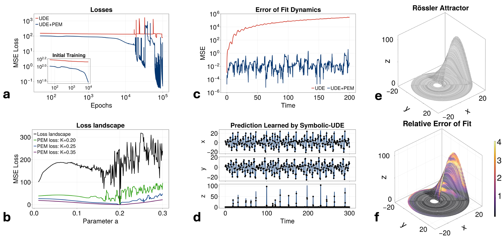
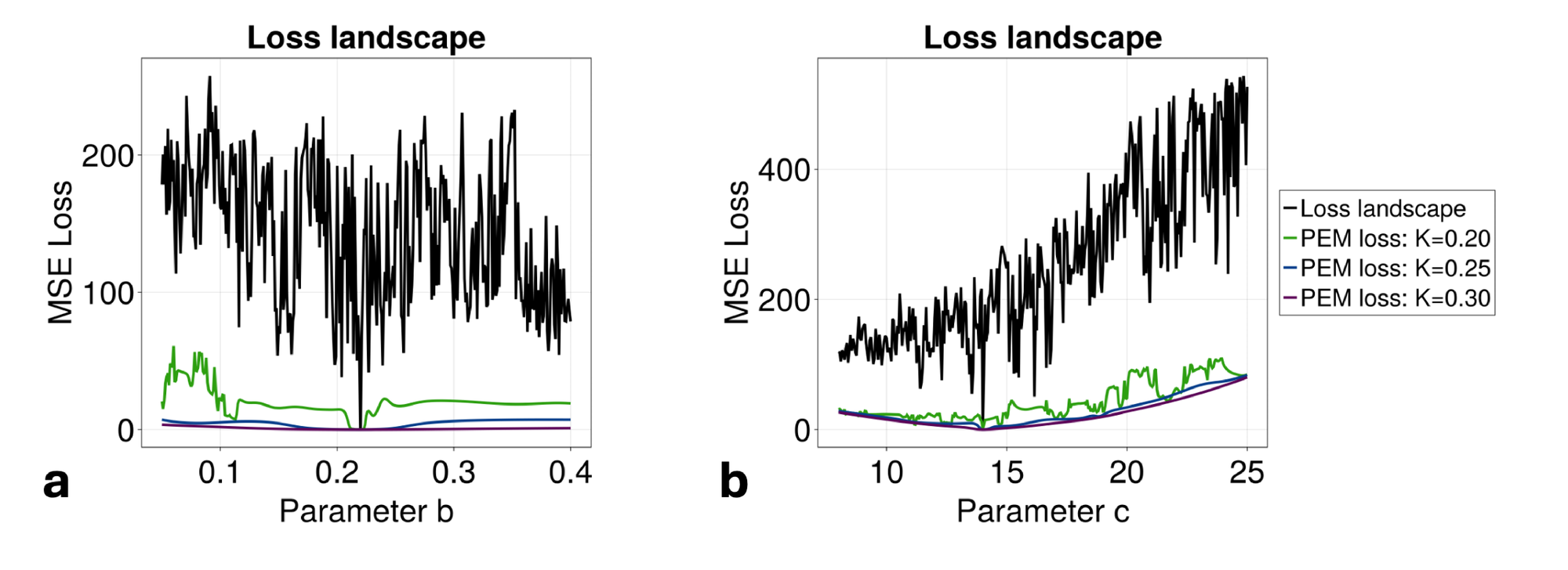
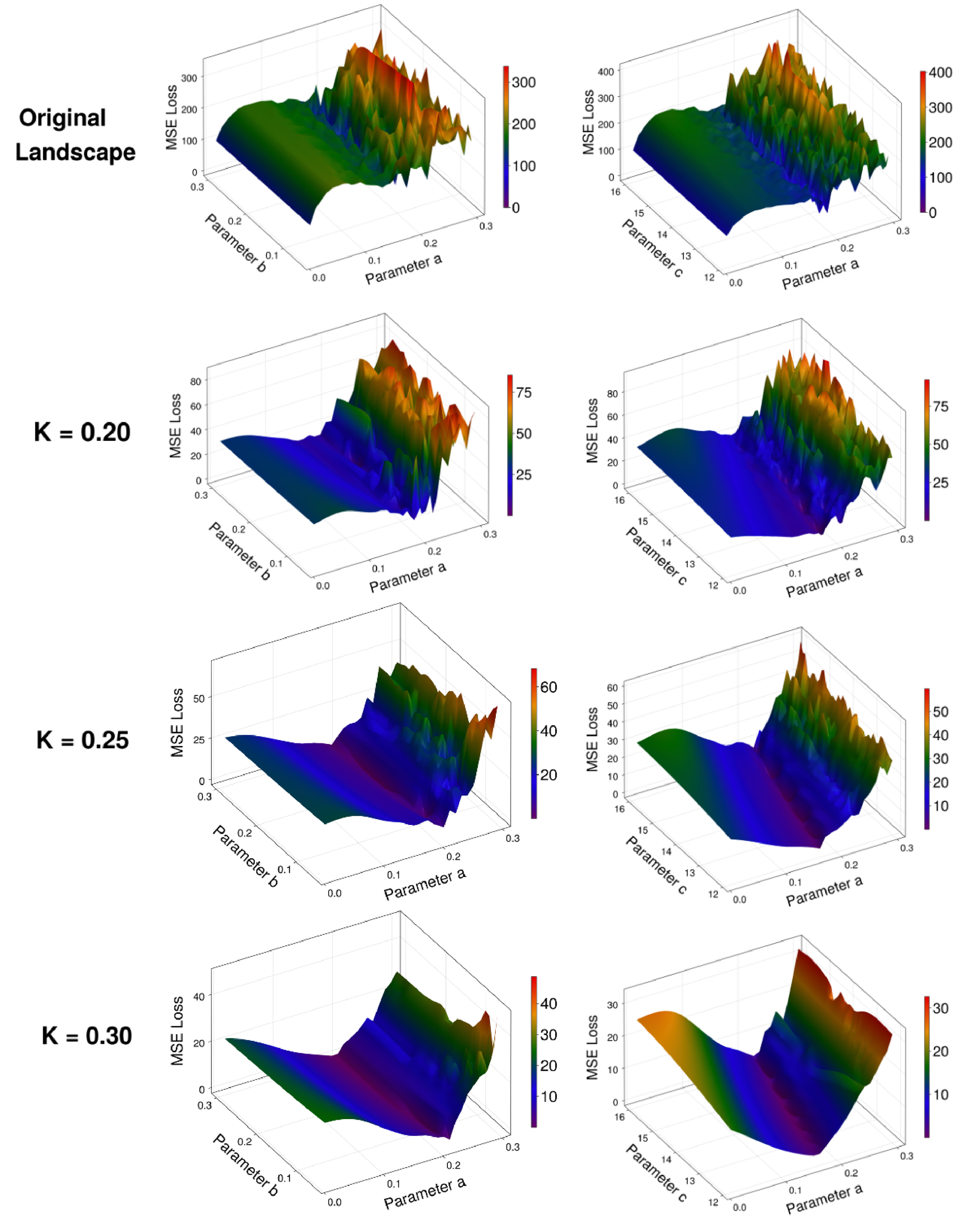
The reason for this performance increase lies in the way that the PEM approach alters the landscape over which the UDE is being trained (Fig. 2b). We note that the unmodified landscape is extremely rough and contains several local minima, with only a very sharp decrease in loss at the true global minimum (\( a=0.2\) in this case). By adding the PEM to the dynamics of the system during training of the UDE, the landscape becomes much more approachable via standard optimization techniques. Further, the choice of \( K\) can be made to directly tune the steepness of the landscape. This should be done in conjunction with considering how the PEM will smooth out the landscapes of other parameters in states where the PEM is not applied. For reasonable choices of \( K\) , the addition of PEM will not substantially deviate the fit dynamics from the true minima along other parameters (explored more fully in Fig. 6). Importantly, as higher levels of filtering are introduced with larger \( K\) , finding the true functional form of the entire system will rely more upon the accuracy of the estimates of the un-fit parameters (Fig. 7). When using the PEM-UDE combination approach, it is therefore best to select a hyperparameter \( K\) that provides a smooth enough landscape for optimization to occur but is steep enough that the global minimum is still clearly distinguishable from the surrounding area to allow for noisier estimates of unmeasured parameters.
At its core, the PEM-UDE approach works because the prediction error correction removes the sensitive dependence on parameters from the system being fit, effectively negating the hallmark trait of chaotic systems. As shown in Fig. 9a, when \( K\) is small there is an \( \mathcal{O}(1)\) divergence with respect to any deviation in the initial parameter choice (illustrated as a deviation of 1e-9 in Fig. 9a), but as \( K\) is sufficiently large (\( K\approx0.18\) in this example) this sensitive dependence is eliminated and the error between the two trajectories shrinks. For sufficiently large \( K\) , this error will depend on the size of the deviation in the parameter, and \( K\) can be tuned based on the estimate of this deviation (Fig. 9b). This property, along with the fact that when the error term in Eq. 6a shrinks to zero the dynamics of the original system are fit, means that the PEM perturbed system is well-behaved (i.e. non-chaotic) and has a loss minimum at the same point as the original system. As such, the L2 norm trajectory fitting approach which is unstable on the original chaotic system is thus stabilized on the PEM-UDE, allowing the fitting process to convergence while leading to an effectively unbiased final fit.
The dynamics learned by the PEM-UDE fit the system well, while the initial estimate of the UDE alone does not offer an accurate prediction even within the Lyapunov time of the system (Fig. 2c). For the parameters selected here, the Lyapunov time of the system is \( \lambda^{-1} \approx 10\) , with most nearby areas of parameter space having similar characteristic times (\( \lambda^{-1} < 25\) ; see Methods for more details). While the mean error of the UDE alone continues to grow throughout the simulation time, the mean error at each timestep of the PEM-UDE fit dynamics is 2-3 orders of magnitude smaller than the dynamics themselves.
To generalize these dynamics beyond the original observations, we extracted a symbolic form of the equations using STLSQ fit to the dynamics of the PEM-UDE system and the outputs of the UDE at each timestep. The functional form of the missing state is directly recovered by STLSQ (\( y = p_1x + p_2y\) ), with the initial fits of parameters close to the true values (\( p_1 = 1.01\) , \( p_2=0.17\) , while the true values are \( p_1=1\) , \( p_2=0.2\) ). By adding an additional optimization step to tune the parameters of this learned symbolic equation after STLSQ, we are able to converge to the true values (accurate to three decimal places), which then generalize the dynamics forward in time beyond the original simulations (Fig. 2d). Importantly, this pipeline provides an analytical form of the dynamics that not only generalizes forwards in time but can also be interrogated for insights into the physical system.
2.3 PEM-UDE can learn chaotic dynamics even if certain states have limited observational data
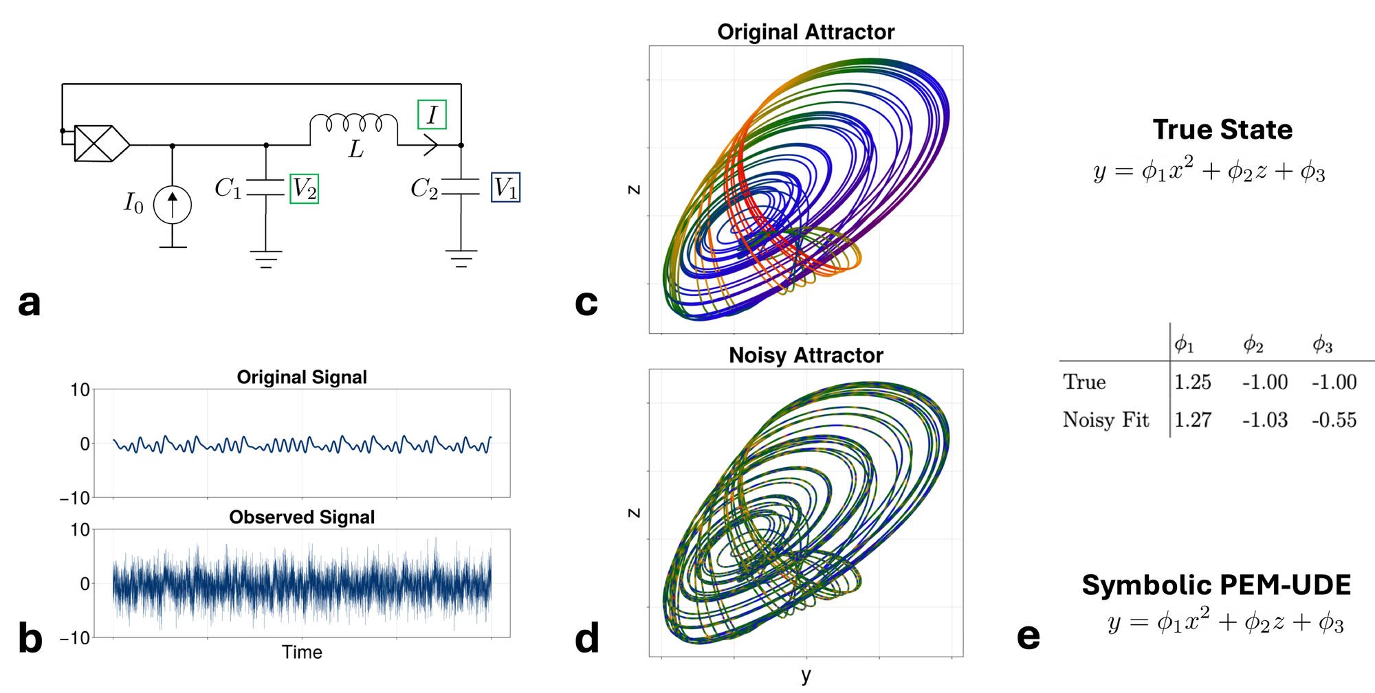
We next present a second example of the PEM-UDE method being fit to a chaotic system, with two important differences compared to the Rössler system. First, this example is one of a physically realized electrical circuit, with the circuit diagram shown in Fig. 3a, and the parameters for the physical circuit (as described in [53]) given in 2. Conceptually, this offers a transition from the idealized chaotic dynamics of the previous system to more real-world applications, as observing chaos in electrical circuits has practical implications [54]. To extend our method further, we create a second challenge – adding a noisy observation to one of the circuit components (\( V_1\) , denoted by the red box shown in Fig. 3a). The true equations for this system are given in 13.a, with the dimensionless form used in this example given by 14.a. In this section, we assume there is an unknown faulty observation of the first state \( x\) , such that there is noise around the observation at 5x the magnitude of the true signal (shown in Fig. 3b). This creates a difficulty for the PEM-UDE fit: the true dynamics (Fig. 3c) are now masked by a significant amount of noise that grossly distorts the shape of the attractor being fit (Fig. 3d).
| \( \lambda\) | Fit expression |
| 0.1 | \( \phi_1 + \phi_2x+\phi_3y+\phi_4z+\phi_5xy+\phi_6y^2+\phi_7xz+\phi_8z^2\) |
| 0.2 | \( \phi_1 + \phi_2x+\phi_3y+\phi_4z+\phi_5xy+\phi_6xz+\phi_7yz+\phi_8z^2\) |
| 0.3 | \( \phi_1+\phi_2y+\phi_3z+\phi_4z^2\) |
| 0.4 | \( \phi_1+\phi_2y+\phi_3z+\phi_4y^2+\phi_5yz\) |
| 0.5 | \( \phi_1+\phi_2y+\phi_3z\) |
We assume that this noise is unknown at the time of fitting and proceed with fitting the PEM-UDE to the corrupted data using the same approach as above (i.e., fitting the functional form shown in 15.a). Despite the significant observational noise present in one of the states, STLSQ applied to the PEM-UDE fit dynamics recovers the exact functional form of the dynamics (Fig. 3e). However, we note that this approach does not provide the original parameters, although the form is correct. In this approach, however, we note that we have shifted the problem from one of unknown dynamics to one of simple parameter optimization, to which other approaches (e.g., simulation-based inference [55]) can be fruitfully applied. This also gives us confidence that even in cases of extremely noisy observational data, the PEM-UDE approach can recover valuable information about the true dynamics of the system.
This example also provides a useful demonstration of why fitting the symbolic form of a trained UDE outperforms a STLSQ fit of the original dataset. As a comparison to the dynamics shown in Fig. 3e, we fit the same noisy dataset directly using the SINDy approach [10, 56], i.e. calculating a dataset of smoothed derivative estimates and performing the STLSQ symbolic regression method directly on the derivative estimates. As shown in Table 1, no recovery of the true symbolic form is possible with this method across a range of the ADMM hyperparameter \( \lambda\) , with more sparse representations incorrectly dropping the noisy state \( x\) from the expression entirely. Recovering the symbolic form of the trained UDE is more accurate as the UDE provides a noise-free (or greatly noise-reduced) version of the dynamics that can be sampled with arbitrary density, thereby mitigating the sensitivity that symbolic regression methods show to noisy data.
2.4 Learning novel expressions for sparse networks that violate original derivation assumptions
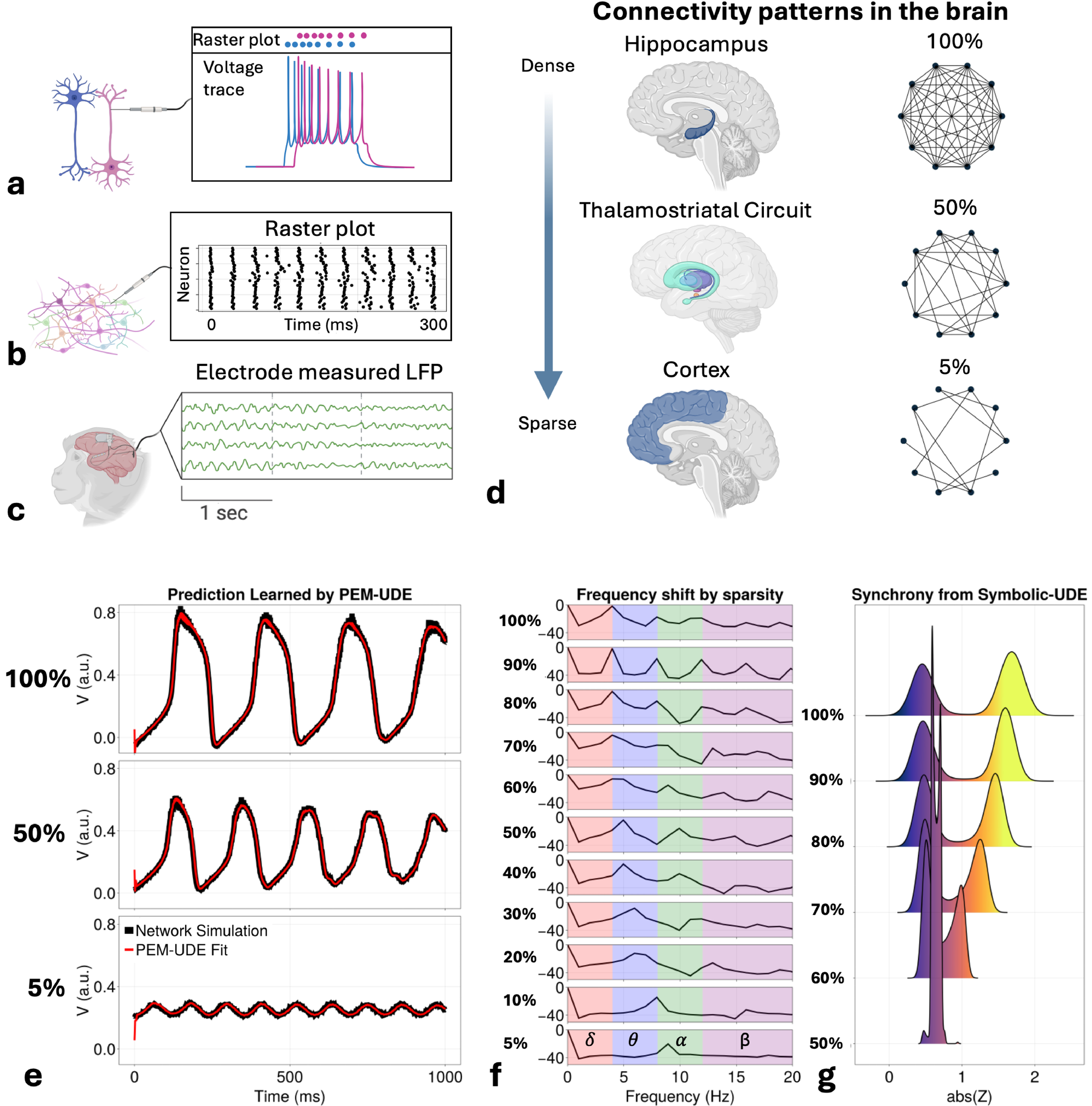
Having demonstrated the utility of this approach in learning forms of chaotic physical systems, we next turn to deriving novel expressions for the mean-field activity of neuron populations. The data needed to study the human brain inherently bridges multiple scales, as individual neuronal activity gives rise to synchronized actions that define interacting functional circuits (Fig. 4a-c). Traditional neural mass models represent the average activity of neuron populations by modeling specific phenomena (e.g., excitatory/inhibitory balance in the Wilson-Cowan model [39], ion gradient dynamics in excitatory populations in the Larter-Breakspear model [41, 57]), but lack a direct tie to many biophysical parameters (e.g., neurotransmitters) that are essential in understanding inter-neuron dynamics. To overcome this, next-generation neural mass models (NGNMMs) take a different approach, providing an analytical derivation of the mean-field dynamics that retains the biophysical details of individual neurons while also capturing the emergent properties at the population level [42, 43]. The derivation and its key assumptions are discussed further in the Methods.
This analytical form of mean-field dynamics offered by NGNMMs provides many advantages over traditional neural mass models. First, there is a direct connection between the single neuron parameters and the dynamics of the neural population, a feature that is only available in certain populations of traditional neural masses tuned to be sensitive to these parameters [41, 57]. Second, NGNMMs capture emergent properties of neural populations that traditional neural masses do not. For example, \( \beta\) -rebound – where the suppressed activity in the \( \beta\) band increases in power after being suppressed (a commonly observed phenomenon in motor cortex studies) – is observed as a feature of coupled NGNMMs that are built only to oscillate in the \( \beta\) band, with no functional constraints that force this activity to occur [44].
Despite these advantages, however, there are some notable limitations to the NGNMM approach, mostly involving the assumptions necessary for the Ott-Antonsen ansatz [45], a key component of the NGNMM derivation. Most important from a biophysical standpoint is the assumption of all-to-all connectivity of the neuron population. This is approximately correct in deep regions (e.g., hippocampus, entorhinal cortex) that have significant within-region collaterals [43]. Immediate neighbors of these regions tend to have fewer collaterals, however, like the thalamostriatal connection patterns [58]. The assumption of full connectivity becomes obviously false in the cortex [48], which typically has very sparse connectivity (on the order of 1-5% of all possible connections; Fig. 4d). Accounting for sparsity in NGNMMs is, therefore, a key problem that must be solved for them to be generalizable in new contexts.
As there is disagreement on the correct analytical approach to adjust the derivation of NGNMMs for sparsity [47, 59, 60], we propose to sidestep the issue of an analytical derivation entirely and simply learn the form of the sparse networks directly from the data with the PEM-UDE method. Following the analytical approach for Izhikevich neurons [43], we begin with a large population of neurons described by Eq. 16 with synaptic dynamics in Eq. 18. In the all-to-all case, the analytical NGNMM describing the activity of this population is given by Eq. 20.a. As we begin to prune connections in the graph to introduce sparsity, however, we see that this form no longer accurately represents the population activity. We therefore learn correction terms for the mean firing rate \( r\) and voltage \( v\) given a reduced probability of connectivity \( p(c)\) , where \( p(c) \in [0.05, 1]\) . Although there are additional states for the recovery current \( w\) and the synaptic dynamics \( s\) , we only learn from the firing rate and voltage states and train only on their data, as these are the data typically available from experiments. Learning directly from these data sources thus allows us to demonstrate the applicability of this approach in learning directly from experimental data.
The PEM-UDE approach is able to capture the mean-field dynamics of the network under different degrees of sparsity to a high degree of accuracy (Fig. 4e). This accuracy does not include the initial conditions; this is discussed further in the limitations and future directions portion of the discussion. It does, however, capture a noticeable shift in the dominant frequency of oscillations present in the network as a function of sparsity (Fig. 4f). Densely connected regions typically have a primary frequency peak in the \( \theta\) -band, while the most sparse networks exhibit a primary peak in the \( \alpha\) -band. This emerges as a natural feature of the learned dynamics and is also observed in experimental data. Hippocampal rhythms are typically in \( \theta\) frequencies and emerge from the densely connected areas of the brain [61], while \( \alpha\) frequencies typically emerge from sparsely connected cortical regions before propagating through the brain [62]. The PEM-UDE learned dynamics therefore preserve and extend the strength of NGNMMs in capturing the emergent properties (e.g., synchrony) at the mean-field scale by accurately captuging the ergodic properties of the system.
As in the previous two systems, we extend the PEM-UDE learned dynamics described in Eq. 22.a by fitting a symbolic form of the dynamics to the UDE network with STLSQ, providing an analytical form of the solution (shown in Eq. 23.a, with fit parameters in Table 4). As NGNMMs are derived based on the assumption of a population of coupled oscillators, there is an exact expression for the degree of synchrony within the population given by the expression for the Kuramoto order parameter \( Z\)
(7)
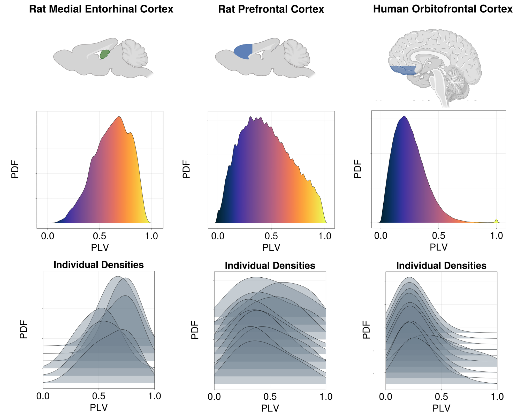
In the case of the symbolic form of the PEM-UDE learned network dynamics, we observe an emergent prediction that more densely connected regions will tend to have higher degrees of synchrony as a baseline state. In comparison, more sparsely connected regions will tend to exhibit lower degrees of synchrony when not acted upon by an external drive (Fig. 4g). This forms an interesting and unexpected prediction from the discovered equations for networks of different sparsity. To test the validity of this prediction, we examined three different datasets of intracranial electrode recordings from regions of different degrees of sparsity (Fig. 5). These datasets included recordings from the rat medial entorhinal cortex (MEC; N=6), a deep region near the hippocampus with high intraregional connectivity [63, 64]; the rat prefrontal cortex (N=10), which has significantly sparser connectivity [65, 66]; and human orbitofrontal cortex (N=10), which exhibits a similarly high degree of sparsity [67, 68]. As predicted by the discovered equations, we note that the deeper, more densely connected structures exhibit a higher degree of synchrony than either of the cortical datasets, and this is a broad trend across individuals, although there is significant variability between subjects. These results suggest that the learned equations are not merely capturing the dynamics on which they are trained but have been able to predict features beyond their initial training data, indicating a more general applicability than the original form allowed.
3 Discussion
Here, we introduce a new method to fit universal differential equations in chaotic systems and demonstrate that it learns novel governing equations for neural population activity. The approach harnesses the prediction error method to train the UDE system, from which we then extract a symbolic form of the learned dynamics via symbolic regression [10]. We demonstrate that our method can learn the dynamics of a classical chaotic system, using the Rössler system [22]. A standard UDE alone cannot learn this system effectively. However, our combined PEM-UDE approach captures the dynamics accurately, demonstrating that our method has identified the true functional form of the dynamics rather than merely making projections within conventional statistical boundaries. Prior work in UDEs has focused on stiff systems [7], fitting UDEs in the presence of stochastic noise [69], and extracting explainable functions from UDE networks [16]. Independently, prior work in parameter optimization using the PEM has shown its utility in fitting parameters of dynamical systems [17, 52], and has shown that it can even outperform neural network fits of dynamics [70, 71]. Our approach here represents the first time the PEM has been used to train UDEs and to extract a functional form of these UDEs to provide an analytical result. Our approach succeeds where standard UDE methods fail because it effectively smooths the parameter landscape the UDE must optimize. Importantly, this smoothing removes a sensitive dependence on the parameters of the system while retaining a loss minimum at the same value as the original system, creating a well-behaved problem when fitting the dynamics. We also extend this application to a second chaotic system from an electrical circuit [72, 53], and show that even in the presence of significant observational noise, the PEM-UDE method can recover the true functional form of an unknown state. A more accurate estimation of the parameters of these recovered dynamics could be achieved by taking the functional form learned from the PEM-UDE dynamics and applying a more advanced optimization technique that fully uses the ability to simulate the system in different regimes (e.g., simulation-based inference [55]).
Having shown that the PEM-UDE approach can learn the dynamics of chaotic systems, we then consider how to learn governing equations in systems of neurons under biologically plausible constraints. These constraints are of two varieties: experimental constraints on the data available, including using only data sources that can be feasibly acquired in vivo (firing rate, membrane voltage); and neurobiological, where the sparsity of interneuron connections can be accurately modeled. Experimental constraints are useful to bear in mind as they can make the method more immediately applicable, but advances in methods can often relax these constraints over time. Biological constraints, and connection density in particular, are more important to accurately model, as they fulfill an important role in the types of information processing possible within the brain [49, 50]. We use a missing-physics approach, where the initial form of the population activity is given by a next-generation neural mass model [42, 43]. NGNMMs have shown great promise in capturing emergent properties of neuron populations while retaining the microscale parameters that are typically manipulated in vitro [44, 73], but rely on the assumption of all-to-all connectivity that is inherently non-physiological for most brain regions [42]. There have been varied attempts to sidestep this limitation and include corrections for sparsity by reweighting the degree of synaptic conductance or the distribution of synaptic currents, with varying degrees of success [47, 59, 74, 60]. Each of these approaches comes with new assumptions and its own limitations. Here, we avoid this by learning a novel NGNMM as the governing equation for a population of Izhikevich neurons directly from the observations of the network itself. We demonstrate that the governing equations learned by this approach predict novel emergent properties that are observed directly in biology, like the shift from \( \theta\) to \( \alpha\) as the dominant frequency band as networks become more sparse – a feature seen in the brain moving from densely connected regions (e.g., hippocampus) to sparsely connected regions (e.g., prefrontal cortex) [61, 62]. These governing equations also predict that more densely connected regions will exhibit greater intraregional synchrony at rest than sparsely connected networks. To test this hypothesis, we compute the intraregional synchrony from three datasets of intracranial electrode recordings (rat MEC, rat prefrontal cortex, and human orbitofrontal cortex) [63, 65, 67]. Across all datasets, we see that the pattern predicted by the discovered equations holds true: intraregional synchrony at rest is inversely correlated with the degree of connectivity between neurons in the region, giving us further validation that the PEM-UDE method is capable of uncovering equations that accurately describe complex biological systems.
Despite its strengths, the method presented here also has limitations that will be addressed in future work. Extremely noisy systems can be difficult to learn, especially as chaotic systems can be complicated to average over trials. Additionally, care must be taken because it is possible that nonphysical solutions also shadow physical ones [24]. The inclusion of information during training via the PEM and the extraction of a symbolic form of the dynamics help mitigate these difficulties. In models that include known physics, PEM can lead to close-but-inaccurate minima if the parameters are not exactly known. This limits the method’s applicability to scenarios where the parameters included in the known physical model are sufficiently accurate. In principle, this can be overcome by also fitting to a range of simulations across these parameters, but the training time will be significantly increased. Finally, the method presented here is best suited for situations with a known structure of data (i.e., some driving inputs are known). Neural experiments frequently provide this level of accuracy, but there is also substantial interest in resting state data [75]. Adapting our approach to accurately fit stationary time series without known perturbations is thus also an important extension for neuroscience applications.
Although the work presented here demonstrates the significant utility of this approach in neuroscience, there are notable areas for further development. Future work can incorporate loss objectives that include optimization of initial conditions, as this can assist in generalization to real-world systems [70, 76]. Future work can also focus on learning "black-box" representations of the dynamics, where symbolic regression methods are not applied to learn the dynamics. This can be useful in situations where complexity penalties (i.e., enforced sparsity within the learned expression) bias away from the correct dynamics. For example, in a case where many small inputs lead to complex interactions based on their temporal pattern, the high-dimensional representation present in the neural network may be more desirable. The temporal sequences of visual cortex projections to the prefrontal cortex are an example of this kind of structured high-dimensional input space [48]. In such a case, rather than fitting the dynamics symbolically, a second optimization run of the UDE without PEM after the initial combined run could lead to more generalizable results (as this forces the contribution of PEM to 0 rather than just naturally minimizing it over the optimization problem). Including a method for directly estimating stochastic processes within the dynamics, as has been done in some standard UDE approaches [69], would provide an additional layer of generalization to this approach. Finally, extending the PEM-UDE approach to systems of partial differential equations would allow for a direct fitting of neural field models under differing degrees of connection density, which are of increasing importance as neuroscience begins to understand the importance of traveling waves in the brain [77, 19] and how the interplay between densely and sparsely connected regions structures the flow of cognitive processes [49].
4 Methods
4.1 Scientific machine learning in the Julia ecosystem
The Julia ecosystem has a robust infrastructure for scientific machine learning [16] that we use to build the PEM-UDE method described in this work. As setting up and training UDEs in Julia has been discussed in other publications ([16, 7] are notable examples), we encourage interested readers to simply peruse the code to see the details of the implementation and content ourselves with a few brief technical notes here on details about the choices of solvers, network structure, fitting procedure, and symbolic regression.
In this work, we default to non-stiff solvers (typically Vern7), largely for speed considerations. As long as the UDE network is sufficiently large to allow for a decent approximation of the unknown dynamics and the system itself is not incredibly stiff, a non-stiff adaptive solver should provide sufficiently accurate fits to the dynamics. If the system is known or highly suspected to contain a great deal of stiffness, then switching to a stiff solver (e.g., FBDF) is recommended and is easy to do in the provided code, as the Julia ecosystem has a wide range of solvers available. This switch may become necessary either because chaotic systems are often stiff in areas, or even if the system itself is not stiff (as the neural systems discussed can be in the correct parameter space), the inclusion of a universal approximator will often lead to a stiff problem, at least until the initial parameter weights are adjusted to fit the problem. We recommend increasing the size of the universal approximator network before defaulting to a stiff solver, as this can significantly impact performance.
We choose the radial basis function (RBF; notation given in [78]) as the activation function for these layers, given by
(8)
The RBF is selected for both theoretical and practical reasons. There is a robust body of literature showing that the RBF is useful in the context of universal approximation [78, 79, 80]. Because a neural network of this form can approximate any function given a sufficient depth of the network [78], the choice of network size is therefore arbitrary beyond a specific size. It can be set freely based on the availability of computational resources for training. For the networks shown in this work, we choose a depth of four layers, where for an input dimension \( N_1\) and output dimension \( N_2\) , each network is of size \( N_1 \times 10 \times 10 \times N_2\) .
As the PEM portion of training requires interpolating the original training data to the solver time step, we use DataInterpolations.jl to do simple linear interpolation between observations [81]. Although there are many optimizers provided to train the UDEs, we have defaulted to using the AdamW method (decoupled weight decay and gradient updates; [82]) in all of the results presented here.
While the dynamics fit by the combined PEM-UDE method appear to capture the true dynamics of the system, it is important to note that they are trained on limited data, and evaluating robustness – particularly in chaotic systems with their sensitivity to initial conditions – is challenging to carry out. The approach to mitigating this is to fit a symbolic expression to the dynamics of the UDE networks that we train to provide a form of the dynamics that can be interrogated with standard analytical approaches. For the purposes of this paper, we do not make any claims as to the best way of extracting the symbolic form of the UDE network and note that there are advantages to different approaches [3]. We provide examples of two of these approaches [10, 14] in the code repository associated with this work. As the STLSQ approach is significantly faster than the genetic algorithm approach when large amounts of data (\( N \gtrapprox 10,000\) data points) are required to fit the functional form accurately [14], we default to this method for the results shown here. In principle, however, the trained UDE can be used to generate a subsample of arbitrary density, so either approach can be used, depending on the requirements of the problem at hand.
The notation for the symbolic recovery of terms from neural networks is adapted from [10], so we briefly explain it here. \( \Theta\) is defined as the feature library with some linear combination of features given by weights \( \xi\) so that \( y=\Theta\xi\) . To reduce the library components that constitute the functional form, a sparse solution is found via LASSO [83]. The objective function is therefore given by
(9)
In the implementation used in this work, this objective is approximated by sequential thresholded least-squares (STLSQ) solved for using the alternating direction method of multipliers (ADMM; [84]), as implemented in DataDrivenDiffEq.jl [56].
4.2 Background on the Rössler system
The Rössler system is a set of three nonlinear differential equations as a simplified model for studying chaotic dynamics, as it contains only one nonlinear term but still generates complex chaotic behavior. The dynamics of the system are described by the 3D ODE system:
(10.a)
For specific parameter values (in the case presented here, \( a=0.2\) , \( b=0.22\) , \( c=14\) ), it produces the distinctive funnel-shaped Rössler attractor that exhibits sensitivity to initial conditions, fractal structure, and period-doubling chaotic activity. We chose this as an initial demonstration of the ability of PEM-UDE combination learning as, despite its simplicity, the Rössler system demonstrates essential chaotic properties including positive Lyapunov exponents, topological entropy, and various bifurcation sequences that have helped researchers understand transitions between ordered and chaotic regimes in dynamical systems. Additionally, the Rössler system has been extended to analytically describe certain physical problems (e.g., mechanical vibrations, atmospheric variability).
In the results presented here, we use a universal approximator \( U\) to learn the dynamics of the entire second state, assisted by the Kalman-filtered observational data through the PEM technique. The system simulated during learning is therefore given by
(11.a)
For the results presented in the main text, we select \( K=0.25\) . This choice is driven by the steepness of the parameter landscapes as discussed in the results, and other reasonable values of this hyperparameter will not affect the accuracy of the learned dynamics, provided an appropriate solver is chosen. The results presented here are based on 100,000 training epochs with the AdamW optimizer [82]. The loss function used to train the UDE network is simply mean-squared error between the predicted states at each time step and the true time series (with a small amount of noise added for robustness during training):
(12)
For the parameters selected in our analyses, we characterized the degree of chaos via the Lyapunov time of the system as \( \lambda^{-1} \approx 10\) . Most parameter combinations in the surrounding space have similar values (\( >80\%\) have \( \lambda^{-1} \in [0, 25]\) - see supplemental code for computation of the empirical CDF of the maximum Lyapunov exponents). Lyapunov exponents were computed using standard functions offered in ChaosTools.jl [85, 86].
4.3 Background on Petrzela-Polak circuit
Petrzela and Polak [72] introduced a category of analog electrical circuits exhibiting chaotic dynamics under three constraints: a canonical form, structurally stable attractors, and novel dynamics. Here, we work with a particular realization that provides chaotic dynamics that are visually interesting and can be physically realized in a simple circuit, with the attractor seen on an oscilloscope (demonstrated in [53], from which we take the parameters and non-dimensional form discussed here). For the circuit shown in 3a, the equations describing the three observed states are given by
(13.a)
(13.b)
For convenience in numerical simulations, we work with the non-dimensional form of the system (i.e., one in which physical constants are replaced with the minimal number of parameters to represent the same dynamics). The non-dimensional form of this system is given by
(14.a)
(14.b)
All parameters for both the dimensional and dimensionless systems are taken from [53], and are provided in Extended Data Table 2.
| Parameter | Value |
| \( R_L\) | 0.5k\( \Omega\) |
| \( R_M\) | 0.08k\( \Omega\) |
| \( C_1\) | 1.0\( \mu\) F |
| \( C_2\) | 1.0\( \mu\) F |
| \( L\) | 1.0H |
| \( I_0\) | 1.0mA |
| Dimensionless Parameters | |
| \( a\) | 1.25 |
| \( b\) | 0.5 |
| \( c\) | 1.0 |
The form of the equations learned by the PEM-UDE method is given by:
(15.a)
(15.b)
The loss function used to train this PEM-UDE combination is the same as 12 to demonstrate the robustness of the system to a poorly observed state. If it is known a priori that the observations of a state are corrupted to that degree, it could be worth modifying the loss specified in 12 to weight the error in this state less during training or to drop the observations altogether. As shown in the next section, the PEM-UDE training method can recover dynamics even when some states are completely hidden, provided the initial guess of their dynamics is sufficiently accurate.
4.4 Spiking neural networks and next-generation neural mass models
Next-generation neural mass models rely on the Ott-Antonsen (OA) ansatz to derive the mean-field activity of a population of neurons [45, 42]. Briefly, this approach was introduced as a means of bypassing the need to set up an entire Fokker-Planck equation to derive the mean-field activity of a population of coupled oscillators, provided certain key assumptions are met. The OA ansatz [45] relies on the assumption that the population of coupled oscillators being examined exists in the thermodynamic limit (i.e., \( N \rightarrow \infty\) ) and that the probability distribution of the observable (typically voltage) in phase space converges to a Lorentzian. However, this derivation can approximate other distributions to a reasonable degree of accuracy [47]. The OA ansatz approach also assumes that the noise input into each neuron receives a heterogeneous, quenched noise input \( \eta\) drawn from a general distribution. The key point of this assumption is that the currents cannot be stochastic; otherwise, the prior assumption (the Lorentzian ansatz) is violated, which is further discussed below. The OA ansatz also assumes that the conditional probabilities of the macroscopic variables are separable. This assumption and its limitations have been discussed at length [74], and a second-order circular cumulant approximation has been derived for neural mass models [59]. Finally, the OA ansatz makes the assumption we address in this paper: The network being approximated has an all-to-all connectivity structure. As we have discussed above, this is a fundamentally non-physiological assumption for most regions of the brain, and removing this assumption is an important step in developing more accurate neural mass models.
As we do not require the OA ansatz for the work presented here beyond the initial assumption of the functional form for population activity that will be used to train the UDE, we omit most of the derivation and discuss only the key points. The equations shown here are adapted from earlier work that shows the entire derivation [43]. Following this work, we simulate a network of Izhikevich neurons that take the form
(16)
(17)
where \( V_j\) and \( w_j\) are the voltage and recovery current, respectively, of neuron \( j \in [1,N]\) for a network of \( N\) neurons. The voltage activity in these neurons depends on the internal neuronal dynamics, the distributed noise source \( n_j\) described above, any external driving current \( I_\text{ext}\) , and the synaptic current from other interneuronal connections \( I_{\text{syn},j}\) . The synaptic activity is given by
(18)
(19)
Each neuron therefore receives an impulse of \( \frac{s_\text{jump}}{N}\) at every time that a presynaptic neuron \( k\) fires. If the network is structured to fulfill the assumptions discussed above, the mean-field activity of the entire poulation can be derived using the OA ansatz and will take the form:
(20.a)
(20.b)
where \( r\) is the population firing rate, \( v\) is the mean voltage, \( w\) the mean recovery current, and \( s\) the mean synaptic activity. As discussed in earlier work, this is an accurate representation of the mean-field activity for fully connected networks [43].
For all the simulations presented here, we simulate a network of 1,000 Izhikevich neurons with varying degrees of network sparsity, where the probability of two neurons forming a synapse is given by \( p(c) \in[0.05, 0.1, 0.2,...1.0]\) as indicated for the sparsities shown in Fig. 4. In a standard network of neurons, as the sparsity of connections is varied, it is necessary to rescale the synaptic currents proportionally with the median in-degree of connectivity \( K\) to maintain balanced (synchronous) activity. Previous work has shown that rescaling the synaptic conductance with \( g \propto \frac{1}{\sqrt{K}}\) – with similar rescaling of background currents, if present – provides an accurate scaling for a broad spectrum of network arrangements (in-degrees with Lorentzian, Gaussian, and Erdős-Rényi distributions) [47]. Following this work, we rescale synaptic conductance with \( p(c)\) such that
(21)
As in the previous sections, we set up the UDE to learn the unknown terms for the states we are interested in, but with two key differences. We are learning terms for both the first and second states in this derivation and thus applying PEM to both of these states as well. We also modify Eq. 12 to train on only data for the first two states, as these are the only states typically observable in experimental data. The initial parameters for this system are given in Table 3, and the formal description of the PEM-UDE system is given by
(22.a)
(22.b)
After learning the dynamics with the PEM-UDE approach and recovering the symbolic form of the UDE expressions via STLSQ, the new NGNMM with correction factors for sparsity is given by the parameter values in Table 4 and by the functional form:
(23.a)
(23.b)
| Parameter | Value | Interpretation |
| \( \alpha\) | 0.6215 | Dimensionless Izhikevich voltage parameter |
| \( g_\text{syn}\) | 1.2308 | Synaptic conductance |
| \( I_\text{ext}\) | 0 | External current |
| \( e_r\) | 1 | Synaptic reversal potential |
| \( a\) | 0.0077 | Dimensionless Izhikevich recovery current parameter |
| \( b\) | -0.0062 | Dimensionless Izhikevich recovery current parameter |
| \( w_\text{jump}\) | 0.0189 | Recovery current update per spike |
| \( \tau_s\) | 2.6 | Synaptic time constant |
| \( s_\text{jump}\) | 1.2308 | Synaptic activity update per spike |
| \( v_\text{peak}, v_\text{reset}\) | 200 | Cutoffs for \( v_\infty\) |
| \( \bar{\eta}\) | 0.12 | Mean of Lorentzian for applied noise currents |
| \( \Delta\) | 0.02 | Width of Lorentzian for applied noise currents |
| Parameter | Value | Interpretation |
| \( \phi_1\) | -0.45 | Reduction of synaptic activity contribution to firing rate |
| \( \phi_2\) | -0.20 | Reduction of mean firing rate as connectivity decreases |
| \( \phi_3\) | 0.55 | Increased voltage contribution to firing rate as connectivity decreases |
| \( \phi_4\) | 0.89 | Increased contribution of firing rate to voltage |
| \( \phi_5\) | 1.72 | Starkly increased contribution of recovery current to voltage |
| \( c_1\) | 0.17 | Rescaling of \( \Delta\) |
| \( c_2\) | -0.14 | Rescaling of \( \bar{\eta}\) |
4.5 Experimental data acquisition and preprocessing
As acquisition and preprocessing of each of the three experimental datasets have been described in detail in their respective publications [63, 65, 67], we only briefly describe the datasets here. The rat MEC dataset [64] was acquired from six male Long-Evans rats, with electrode recordings acquired during a long period of roaming in a circular track. The rat prefrontal cortex dataset [66] was acquired from four male Long-Evans rats during 10 trials in which they successfully learned a behavioral task, including the rest periods before and after the task recordings. The human orbitofrontal cortex dataset [68] was acquired during electrocorticography recordings of 10 neurosurgical patients undergoing evaluation for epilepsy. The patients were asked to play a decision-making game, and the recordings used for this data are the inter-trial rest portions of the ECoG data. For all datasets, the synchrony between electrodes within the region was computed as the phase-locking value (PLV) between the angle of Hilbert-transformed signals (\( \phi\) ) from each electrode [87, 88]. Following prior work [48], spike data from the dataset, which recorded spike times rather than LFPs, were converted to an LFP proxy by windowed spike counts, with the PLV calculation performed on these instead. PLV is given by the formula
(24)
for all discretized \( t \in [1, N]\) and all pairs of electrodes \( (i, j)\) .
5 Acknowledgments
We thank Alex Driussi and Botond Antal for their valuable support with graphics. The research presented here was funded by the Baszucki Brain Research Fund, United States (LRMP). AGC also acknowledges the NIHGM MSTP Training Award, United States (T32-GM008444).
6 Code and Data Availability
All code and simulated data to reproduce the results and plots in this manuscript, along with an additional abbreviated demo version for interested readers to rapidly prototype with, can be found in the GitHub repository associated with this publication at https://github.com/Neuroblox/pem-ude. The intracranial electrode recording datasets can all be accessed in repositories on https://crcns.org/, with the specific conditions of access to each one listed on their individual repository pages [1, 2, 3].
7 Competing Interests
The authors declare the following competing interests: authors C.V.R., E.K.M., R.H.G., A.E., L.M.P., and H.H.S. are co-founders of Neuroblox Inc., a company spun out of SUNYSB, MIT, and Dartmouth to develop a commercial-grade software platform for multi-scale computational neuroscience with applications to diagnosis and treatment of brain-based disorders.
8 Supplemental Information
Four supplemental figures: Fig. 6 for a complete description of the method presented here, Fig. 7 for the supplemental parameter profiles of the Rössler system under PEM, Fig. 8 for the 2D parameter landscapes of the Rössler system under PEM and Fig. 9 for the influence of PEM on the divergence of shadow trajectories.
One supplemental table: Table 1 for the STLSQ fits directly to the noisy data.
![Sufficiently large hyperparameter K) for the PEM removes sensitive dependence on initial parameter values. <span style="font-weight: 700">a. The trajectories of the Rössler system diverge for two very close parameter values ( a=0.2) vs a=0.200000001) ), but this divergence is mitigated by sufficiently large K) in the PEM correction term. <span style="font-weight: 700">b. This correction provides the same aid to fitting for any reasonable deviation from the true parameter (shown for deviations in the range [1e-12, 1e-1].](../../media/Scientific-Machine-Learning-of-Chaotic-Systems-Discovers-Governing-Equations-for-Neural-Populations/figs4.png)
References
[1] Distilling Free-Form Natural Laws from Experimental Data Science 2009 324 5923 81--85 apr Publisher: American Association for the Advancement of Science 10.1126/science.1165893
[2] M. Schmidt and H. Lipson, Distilling Free-Form Natural Laws from Experimental Data, https://doi.org/10.1126/science.1165893 Science 324, 81 (2009), publisher: American Association for the Advancement of Science
[3] The automation of science Science 2009 324 5923 85--89 Publisher: American Association for the Advancement of Science
[4] R. D. King, J. Rowland, S. G. Oliver, M. Young, W. Aubrey, E. Byrne, M. Liakata, M. Markham, P. Pir, L. N. Soldatova, and others, The automation of science, Science 324, 85 (2009), publisher: American Association for the Advancement of Science
[5] Discovering Symbolic Models from Deep Learning with Inductive Biases NeurIPS 2020 14 in https://proceedings.neurips.cc/paper/2020/hash/c9f2f917078bd2db12f23c3b413d9cba-Abstract.html
[6] M. Cranmer, A. Sanchez-Gonzalez, P. Battaglia, R. Xu, K. Cranmer, D. Spergel, and S. Ho, Discovering Symbolic Models from Deep Learning with Inductive Biases, in https://proceedings.neurips.cc/paper/2020/hash/c9f2f917078bd2db12f23c3b413d9cba-Abstract.html NeurIPS 2020 (2020) p. 14
[7] The physics of cooperative transport in groups of ants Nature Physics 2018 14 7 683--693 jul Publisher: Nature Publishing Group 10.1038/s41567-018-0107-y
[8] O. Feinerman, I. Pinkoviezky, A. Gelblum, E. Fonio, and N. S. Gov, The physics of cooperative transport in groups of ants, Nature Physics 14, 683 (2018), publisher: Nature Publishing Group
[9] Neural general circulation models for weather and climate Nature 2024 632 8027 1060--1066 aug Publisher: Nature Publishing Group 10.1038/s41586-024-07744-y
[10] D. Kochkov, J. Yuval, I. Langmore, P. Norgaard, J. Smith, G. Mooers, M. Klöwer, J. Lottes, S. Rasp, P. Düben, S. Hatfield, P. Battaglia, A. Sanchez-Gonzalez, M. Willson, M. P. Brenner, and S. Hoyer, Neural general circulation models for weather and climate, Nature 632, 1060 (2024), publisher: Nature Publishing Group
[11] A Bayesian Approach to Regional Decadal Predictability: Sparse Parameter Estimation in High-Dimensional Linear Inverse Models of High-Latitude Sea Surface Temperature Variability Journal of Climate 2020 jul Section: Journal of Climate 10.1175/JCLI-D-19-0769.1
[12] D. Foster, D. Comeau, and N. M. Urban, A bayesian approach to regional decadal predictability: Sparse parameter estimation in high-dimensional linear inverse models of high-latitude sea surface temperature variability, Journal of Climate 10.1175/JCLI-D-19-0769.1 (2020), section: Journal of Climate
[13] Stiff neural ordinary differential equations Chaos: An Interdisciplinary Journal of Nonlinear Science 2021 31 9 093122 sep 10.1063/5.0060697
[14] S. Kim, W. Ji, S. Deng, Y. Ma, and C. Rackauckas, Stiff neural ordinary differential equations, Chaos: An Interdisciplinary Journal of Nonlinear Science 31, 093122 (2021)
[15] Multi-scale organization in communicating active matter Nature Communications 2022 13 1 6727 nov Publisher: Nature Publishing Group 10.1038/s41467-022-34484-2
[16] A. Ziepke, I. Maryshev, I. S. Aranson, and E. Frey, Multi-scale organization in communicating active matter, Nature Communications 13, 6727 (2022), publisher: Nature Publishing Group
[17] Game theoretical inference of human behavior in social networks Nature Communications 2019 10 1 5507 dec Publisher: Nature Publishing Group 10.1038/s41467-019-13148-8
[18] N. Pagan and F. Dörfler, Game theoretical inference of human behavior in social networks, Nature Communications 10, 5507 (2019), publisher: Nature Publishing Group
[19] Discovering governing equations from data by sparse identification of nonlinear dynamical systems Proceedings of the National Academy of Sciences 2016 113 15 3932--3937 apr 10.1073/pnas.1517384113
[20] S. L. Brunton, J. L. Proctor, and J. N. Kutz, Discovering governing equations from data by sparse identification of nonlinear dynamical systems, Proceedings of the National Academy of Sciences 113, 3932 (2016)
[21] Using scientific machine learning for experimental bifurcation analysis of dynamic systems Mechanical Systems and Signal Processing 2023 184 109649 feb 10.1016/j.ymssp.2022.109649
[22] S. Beregi, D. A. W. Barton, D. Rezgui, and S. Neild, Using scientific machine learning for experimental bifurcation analysis of dynamic systems, Mechanical Systems and Signal Processing 184, 109649 (2023)
[23] AI Science Advances 2020 6 16 eaay2631 apr Publisher: American Association for the Advancement of Science Section: Research Article 10.1126/sciadv.aay2631
[24] S.-M. Udrescu and M. Tegmark, AI Feynman: A physics-inspired method for symbolic regression, Science Advances 6, eaay2631 (2020), publisher: American Association for the Advancement of Science Section: Research Article
[25] DreamCoder Philosophical Transactions of the Royal Society A: Mathematical, Physical and Engineering Sciences 2023 381 2251 20220050 jun Publisher: Royal Society 10.1098/rsta.2022.0050
[26] K. Ellis, L. Wong, M. Nye, M. Sablé-Meyer, L. Cary, L. Anaya Pozo, L. Hewitt, A. Solar-Lezama, and J. B. Tenenbaum, DreamCoder: growing generalizable, interpretable knowledge with wake–sleep Bayesian program learning, Philosophical Transactions of the Royal Society A: Mathematical, Physical and Engineering Sciences 381, 20220050 (2023), publisher: Royal Society
[27] Interpretable Machine Learning for Science with PySR and SymbolicRegression.jl may 2023 10.48550/arXiv.2305.01582
[28] M. Cranmer, Interpretable Machine Learning for Science with PySR and SymbolicRegression.jl (2023)
[29] Discovering governing equations from partial measurements with deep delay autoencoders Proceedings of the Royal Society A: Mathematical, Physical and Engineering Sciences 2023 479 2276 20230422 aug Publisher: Royal Society 10.1098/rspa.2023.0422
[30] J. Bakarji, K. Champion, J. Nathan Kutz, and S. L. Brunton, Discovering governing equations from partial measurements with deep delay autoencoders, Proceedings of the Royal Society A: Mathematical, Physical and Engineering Sciences 479, 20230422 (2023), publisher: Royal Society
[31] Universal Differential Equations for Scientific Machine Learning arXiv:2001.04385v4 2021 nov arXiv: 2001.04385 https://doi.org/10.48550/arXiv.2001.04385
[32] C. Rackauckas, Y. Ma, J. Martensen, C. Warner, K. Zubov, R. Supekar, D. Skinner, A. Ramadhan, and A. Edelman, Universal Differential Equations for Scientific Machine Learning, arXiv:2001.04385v4 https://doi.org/10.48550/arXiv.2001.04385 (2021), arXiv: 2001.04385
[33] Prediction error estimation methods Circuits, Systems and Signal Processing 2002 21 1 11--21 jan 10.1007/BF01211648
[34] L. Ljung, Prediction error estimation methods, Circuits, Systems and Signal Processing 21, 11 (2002)
[35] Macroscopic models for networks of coupled biological oscillators Science Advances 2018 4 8 e1701047 aug Publisher: American Association for the Advancement of Science 10.1126/sciadv.1701047
[36] K. M. Hannay, D. B. Forger, and V. Booth, Macroscopic models for networks of coupled biological oscillators, Science Advances 4, e1701047 (2018), publisher: American Association for the Advancement of Science
[37] Dynamic models of large-scale brain activity Nat Neurosci 2017 20 3 340--352 feb 10.1038/nn.4497
[38] M. Breakspear, Dynamic models of large-scale brain activity, Nat Neurosci 20, 340 (2017)
[39] Ion gradient-driven bifurcations of a multi-scale neuronal model Chaos, Solitons & Fractals 2023 167 113120 feb 10.1016/j.chaos.2023.113120
[40] A. G. Chesebro, L. R. Mujica-Parodi, and C. Weistuch, Ion gradient-driven bifurcations of a multi-scale neuronal model, Chaos, Solitons & Fractals 167, 113120 (2023)
[41] Effective Latent Differential Equation Models via Attention and Multiple Shooting Transactions on Machine Learning Research
[42] G. Abrevaya, M. Ramezanian-Panahi, J.-C. Gagnon-Audet, P. Polosecki, I. Rish, S. P. Dawson, G. Cecchi, and G. Dumas, Effective latent differential equation models via attention and multiple shooting, Transactions on Machine Learning Research
[43] An equation for continuous chaos Physics Letters A 1976 57 5 397--398 jul 10.1016/0375-9601(76)90101-8
[44] O. E. Rössler, An equation for continuous chaos, Physics Letters A 57, 397 (1976)
[45] Bumps and oscillons in networks of spiking neurons Chaos: An Interdisciplinary Journal of Nonlinear Science 2020 30 3 033133 mar 10.1063/1.5135579
[46] H. Schmidt and D. Avitabile, Bumps and oscillons in networks of spiking neurons, Chaos: An Interdisciplinary Journal of Nonlinear Science 30, 033133 (2020)
[47] On the probability of finding nonphysical solutions through shadowing Journal of Computational Physics 2021 440 110389 sep 10.1016/j.jcp.2021.110389
[48] N. Chandramoorthy and Q. Wang, On the probability of finding nonphysical solutions through shadowing, Journal of Computational Physics 440, 110389 (2021)
[49] What Is an Adjoint Model? Bulletin of the American Meteorological Society 1997 78 nov Section: Bulletin of the American Meteorological Society
[50] R. M. Errico, What is an adjoint model?, Bulletin of the American Meteorological Society 78 (1997), section: Bulletin of the American Meteorological Society
[51] Adjoint sensitivity analysis on chaotic dynamical systems by Non-Intrusive Least Squares Adjoint Shadowing (NILSAS) Journal of Computational Physics 2019 395 690--709 oct 10.1016/j.jcp.2019.06.035
[52] A. Ni and C. Talnikar, Adjoint sensitivity analysis on chaotic dynamical systems by Non-Intrusive Least Squares Adjoint Shadowing (NILSAS), Journal of Computational Physics 395, 690 (2019)
[53] Sensitivity analysis on chaotic dynamical systems by Finite Difference Non-Intrusive Least Squares Shadowing (FD-NILSS) Journal of Computational Physics 2019 394 615--631 oct 10.1016/j.jcp.2019.06.004
[54] A. Ni, Q. Wang, P. Fernández, and C. Talnikar, Sensitivity analysis on chaotic dynamical systems by Finite Difference Non-Intrusive Least Squares Shadowing (FD-NILSS), Journal of Computational Physics 394, 615 (2019)
[55] Least Squares Shadowing Method for Sensitivity Analysis of Differential Equations SIAM Journal on Numerical Analysis 2017 55 6 3030--3046 jan Publisher: Society for Industrial and Applied Mathematics 10.1137/15M1039067
[56] M. Chater, A. Ni, P. J. Blonigan, and Q. Wang, Least Squares Shadowing Method for Sensitivity Analysis of Differential Equations, SIAM Journal on Numerical Analysis 55, 3030 (2017), publisher: Society for Industrial and Applied Mathematics
[57] Least Squares Shadowing sensitivity analysis of chaotic limit cycle oscillations Journal of Computational Physics 2014 267 210--224 jun 10.1016/j.jcp.2014.03.002
[58] Q. Wang, R. Hu, and P. Blonigan, Least Squares Shadowing sensitivity analysis of chaotic limit cycle oscillations, Journal of Computational Physics 267, 210 (2014)
[59] Ergodic theory of chaos and strange attractors Reviews of Modern Physics 1985 57 3 617--656 jul Publisher: American Physical Society 10.1103/RevModPhys.57.617
[60] J. P. Eckmann and D. Ruelle, Ergodic theory of chaos and strange attractors, Reviews of Modern Physics 57, 617 (1985), publisher: American Physical Society
[61] Ergodic Theory Cambridge University Press 1989 nov Google-Books-ID: MiyJGqFCbEMC
[62] K. E. Petersen, Ergodic Theory (Cambridge University Press, 1989) google-Books-ID: MiyJGqFCbEMC
[63] Nonlinear time-series analysis revisited Chaos: An Interdisciplinary Journal of Nonlinear Science 2015 25 9 097610 apr 10.1063/1.4917289
[64] E. Bradley and H. Kantz, Nonlinear time-series analysis revisited, Chaos: An Interdisciplinary Journal of Nonlinear Science 25, 097610 (2015)
[65] Ketamine can produce oscillatory dynamics by engaging mechanisms dependent on the kinetics of NMDA receptors Proceedings of the National Academy of Sciences 2024 121 22 e2402732121 may 10.1073/pnas.2402732121
[66] E. Adam, M. Kowalski, O. Akeju, E. K. Miller, E. N. Brown, M. M. McCarthy, and N. Kopell, Ketamine can produce oscillatory dynamics by engaging mechanisms dependent on the kinetics of NMDA receptors, Proceedings of the National Academy of Sciences 121, e2402732121 (2024)
[67] Achieving Occam's razor: Deep learning for optimal model reduction PLOS Computational Biology 2024 20 7 e1012283 jul Publisher: Public Library of Science 10.1371/journal.pcbi.1012283
[68] B. B. Antal, A. G. Chesebro, H. H. Strey, L. R. Mujica-Parodi, and C. Weistuch, Achieving Occam's razor: Deep learning for optimal model reduction, PLOS Computational Biology 20, e1012283 (2024), publisher: Public Library of Science
[69] Metabolism modulates network synchrony in the aging brain Proc Natl Acad Sci U S A 2021 118 40 oct 10.1073/pnas.2025727118
[70] C. Weistuch, L. R. Mujica-Parodi, R. M. Razban, B. Antal, H. van Nieuwenhuizen, A. Amgalan, and K. A. Dill, Metabolism modulates network synchrony in the aging brain, Proc Natl Acad Sci U S A 118, 10.1073/pnas.2025727118 (2021)
[71] Critical dynamics arise during structured information presentation within embodied in vitro neuronal networks Nature Communications 2023 14 1 5287 aug Publisher: Nature Publishing Group 10.1038/s41467-023-41020-3
[72] F. Habibollahi, B. J. Kagan, A. N. Burkitt, and C. French, Critical dynamics arise during structured information presentation within embodied in vitro neuronal networks, Nature Communications 14, 5287 (2023), publisher: Nature Publishing Group
[73] Theoretical foundations of studying criticality in the brain Network Neuroscience 2022 6 4 1148--1185 oct 10.1162/netn_a_00269
[74] Y. Tian, Z. Tan, H. Hou, G. Li, A. Cheng, Y. Qiu, K. Weng, C. Chen, and P. Sun, Theoretical foundations of studying criticality in the brain, Network Neuroscience 6, 1148 (2022)
[75] A bifurcation integrates information from many noisy ion channels and allows for milli-Kelvin thermal sensitivity in the snake pit organ Proceedings of the National Academy of Sciences 2024 121 6 e2308215121 feb Publisher: Proceedings of the National Academy of Sciences 10.1073/pnas.2308215121
[76] I. R. Graf and B. B. Machta, A bifurcation integrates information from many noisy ion channels and allows for milli-Kelvin thermal sensitivity in the snake pit organ, Proceedings of the National Academy of Sciences 121, e2308215121 (2024), publisher: Proceedings of the National Academy of Sciences
[77] Excitatory and Inhibitory Interactions in Localized Populations of Model Neurons Biophysical Journal 1972 12 1 1--24 jan 10.1016/S0006-3495(72)86068-5
[78] H. R. Wilson and J. D. Cowan, Excitatory and Inhibitory Interactions in Localized Populations of Model Neurons, Biophysical Journal 12, 1 (1972)
[79] Electroencephalogram and visual evoked potential generation in a mathematical model of coupled cortical columns Biological Cybernetics 1995 73 357--366
[80] B. H. Jansen and V. G. Rit, Electroencephalogram and visual evoked potential generation in a mathematical model of coupled cortical columns, Biological Cybernetics 73, 357 (1995)
[81] A coupled ordinary differential equation lattice model for the simulation of epileptic seizures Chaos: An Interdisciplinary Journal of Nonlinear Science 1999 9 3 795--804 sep Publisher: American Institute of Physics 10.1063/1.166453
[82] R. Larter, B. Speelman, and R. M. Worth, A coupled ordinary differential equation lattice model for the simulation of epileptic seizures, Chaos: An Interdisciplinary Journal of Nonlinear Science 9, 795 (1999), publisher: American Institute of Physics
[83] Macroscopic Description for Networks of Spiking Neurons Physical Review X 2015 5 2 021028 jun Publisher: American Physical Society 10.1103/PhysRevX.5.021028
[84] E. Montbrió, D. Pazó, and A. Roxin, Macroscopic Description for Networks of Spiking Neurons, Physical Review X 5, 021028 (2015), publisher: American Physical Society
[85] Exact mean-field models for spiking neural networks with adaptation Journal of Computational Neuroscience 2022 50 4 445--469 nov 10.1007/s10827-022-00825-9
[86] L. Chen and S. A. Campbell, Exact mean-field models for spiking neural networks with adaptation, Journal of Computational Neuroscience 50, 445 (2022)
[87] Next Generation Neural Mass Models Nonlinear Dynamics in Computational Neuroscience Springer International Publishing 2019 Corinto, Fernando and Torcini, Alessandro 1--16 Cham
[88] S. Coombes and A. Byrne, Next Generation Neural Mass Models, in http://link.springer.com/10.1007/978-3-319-71048-8_1 Nonlinear Dynamics in Computational Neuroscience, edited by \bibinfo editor F. Corinto and \bibinfo editor A. Torcini (Springer International Publishing, Cham, 2019) pp. 1--16
[89] Low dimensional behavior of large systems of globally coupled oscillators Chaos: An Interdisciplinary Journal of Nonlinear Science 2008 18 3 037113 sep 10.1063/1.2930766
[90] E. Ott and T. M. Antonsen, Low dimensional behavior of large systems of globally coupled oscillators, Chaos: An Interdisciplinary Journal of Nonlinear Science 18, 037113 (2008)
[91] Discrete Synaptic Events Induce Global Oscillations in Balanced Neural Networks Physical Review Letters 2024 133 23 238401 dec Publisher: American Physical Society 10.1103/PhysRevLett.133.238401
[92] D. S. Goldobin, M. di Volo, and A. Torcini, Discrete Synaptic Events Induce Global Oscillations in Balanced Neural Networks, Physical Review Letters 133, 238401 (2024), publisher: American Physical Society
[93] Transition from Asynchronous to Oscillatory Dynamics in Balanced Spiking Networks with Instantaneous Synapses Physical Review Letters 2018 121 12 128301 sep Publisher: American Physical Society 10.1103/PhysRevLett.121.128301
[94] M. di Volo and A. Torcini, Transition from Asynchronous to Oscillatory Dynamics in Balanced Spiking Networks with Instantaneous Synapses, Physical Review Letters 121, 128301 (2018), publisher: American Physical Society
[95] Biomimetic model of corticostriatal micro-assemblies discovers new neural code jul 2024 10.1101/2023.11.06.565902
[96] A. Pathak, S. L. Brincat, H. Organtzidis, H. H. Strey, S. Senneff, E. G. Antzoulatos, L. R. Mujica-Parodi, E. K. Miller, and R. Granger, Biomimetic model of corticostriatal micro-assemblies discovers new neural code (2024)
[97] Mapping thalamic innervation to individual L2/3 pyramidal neurons and modeling their ‘readout’ of visual input Nature Neuroscience 2023 26 3 470--480 mar Publisher: Nature Publishing Group 10.1038/s41593-022-01253-9
[98] A. Balcioglu, R. Gillani, M. Doron, K. Burnell, T. Ku, A. Erisir, K. Chung, I. Segev, and E. Nedivi, Mapping thalamic innervation to individual L2/3 pyramidal neurons and modeling their ‘readout’ of visual input, Nature Neuroscience 26, 470 (2023), publisher: Nature Publishing Group
[99] Sparse connectivity enables efficient information processing in cortex-like artificial neural networks Frontiers in Neural Circuits 2025 19 1528309 mar Publisher: Frontiers 10.3389/fncir.2025.1528309
[100] R. Fruengel and M. Oberlaender, Sparse connectivity enables efficient information processing in cortex-like artificial neural networks, Frontiers in Neural Circuits 19, 1528309 (2025), publisher: Frontiers
[101] On multistep prediction error methods for time series models Journal of Forecasting 1989 8 4 357--368 _eprint: https://onlinelibrary.wiley.com/doi/pdf/10.1002/for.3980080402 10.1002/for.3980080402
[102] P. Stoica, On multistep prediction error methods for time series models, Journal of Forecasting 8, 357 (1989), _eprint: https://onlinelibrary.wiley.com/doi/pdf/10.1002/for.3980080402
[103] Direct prediction-error identification of unstable nonlinear systems applied to flight test data IFAC Proceedings Volumes 2009 42 10 144--149 jan 10.3182/20090706-3-FR-2004.00024
[104] R. Larsson, Z. Sjanic, M. Enqvist, and L. Ljung, Direct prediction-error identification of unstable nonlinear systems applied to flight test data, IFAC Proceedings Volumes 15th IFAC Symposium on System Identification, 42, 144 (2009)
[105] Elegant Circuits: Simple Chaotic Oscillators World Scientific 2022 feb 10.1142/12362
[106] J. C. Sprott and W. J.-C. Thio, https://doi.org/10.1142/12362 Elegant Circuits: Simple Chaotic Oscillators (World Scientific, 2022)
[107] Hidden attractors in Chua circuit: mathematical theory meets physical experiments Nonlinear Dynamics 2023 111 6 5859--5887 mar 10.1007/s11071-022-08078-y
[108] N. Kuznetsov, T. Mokaev, V. Ponomarenko, E. Seleznev, N. Stankevich, and L. Chua, Hidden attractors in Chua circuit: mathematical theory meets physical experiments, Nonlinear Dynamics 111, 5859 (2023)
[109] Training deep neural density estimators to identify mechanistic models of neural dynamics eLife 2020 9 e56261 sep 10.7554/eLife.56261
[110] P. J. Goncalves, J.-M. Lueckmann, M. Deistler, M. Nonnenmacher, K. Öcal, G. Bassetto, C. Chintaluri, W. F. Podlaski, S. A. Haddad, T. P. Vogels, D. S. Greenberg, and J. H. Macke, Training deep neural density estimators to identify mechanistic models of neural dynamics, eLife 9, e56261 (2020)
[111] DataDrivenDiffEq jul 2021 10.5281/zenodo.5083412
[112] Martensen, Julius, C. Rackauckas, and others, DataDrivenDiffEq.jl (2021)
[113] Modulation of excitatory synaptic coupling facilitates synchronization and complex dynamics in a biophysical model of neuronal dynamics Network: Computation in Neural Systems 2003 14 4 703--732 jan Publisher: Taylor & Francis _eprint: https://doi.org/10.1088/0954-898X_14_4_305 10.1088/0954-898X_14_4_305
[114] M. Breakspear, J. R. Terry, and K. J. Friston, Modulation of excitatory synaptic coupling facilitates synchronization and complex dynamics in a biophysical model of neuronal dynamics, Network: Computation in Neural Systems 14, 703 (2003), publisher: Taylor & Francis _eprint: https://doi.org/10.1088/0954-898X_14_4_305
[115] Thalamic Gating of Corticostriatal Signaling by Cholinergic Interneurons Neuron 2010 67 2 294--307 jul 10.1016/j.neuron.2010.06.017
[116] J. B. Ding, J. N. Guzman, J. D. Peterson, J. A. Goldberg, and D. J. Surmeier, Thalamic Gating of Corticostriatal Signaling by Cholinergic Interneurons, Neuron 67, 294 (2010)
[117] Coherent oscillations in balanced neural networks driven by endogenous fluctuations Chaos: An Interdisciplinary Journal of Nonlinear Science 2022 32 2 023120 feb 10.1063/5.0075751
[118] M. di Volo, M. Segneri, D. S. Goldobin, A. Politi, and A. Torcini, Coherent oscillations in balanced neural networks driven by endogenous fluctuations, Chaos: An Interdisciplinary Journal of Nonlinear Science 32, 023120 (2022)
[119] Exact low-dimensional description for fast neural oscillations with low firing rates Physical Review E 2024 109 1 014229 jan Publisher: American Physical Society 10.1103/PhysRevE.109.014229
[120] P. Clusella and E. Montbrió, Exact low-dimensional description for fast neural oscillations with low firing rates, Physical Review E 109, 014229 (2024), publisher: American Physical Society
[121] Hippocampal theta oscillations are travelling waves Nature 2009 459 7246 534--539 may Publisher: Nature Publishing Group 10.1038/nature08010
[122] E. V. Lubenov and A. G. Siapas, Hippocampal theta oscillations are travelling waves, Nature 459, 534 (2009), publisher: Nature Publishing Group
[123] The generation and propagation of the human alpha rhythm Proceedings of the National Academy of Sciences of the United States of America 2019 116 47 23772--23782 nov 10.1073/pnas.1913092116
[124] M. Halgren, I. Ulbert, H. Bastuji, D. Fabó, L. Erőss, M. Rey, O. Devinsky, W. K. Doyle, R. Mak-McCully, E. Halgren, L. Wittner, P. Chauvel, G. Heit, E. Eskandar, A. Mandell, and S. S. Cash, The generation and propagation of the human alpha rhythm, Proceedings of the National Academy of Sciences of the United States of America 116, 23772 (2019)
[125] Medial entorhinal cortex activates in a traveling wave in the rat eLife 2020 9 e52289 feb 10.7554/eLife.52289
[126] J. J. Hernández-Pérez, K. W. Cooper, and E. L. Newman, Medial entorhinal cortex activates in a traveling wave in the rat, eLife 9, e52289 (2020)
[127] Extracellular recordings from across the dorsoventral axis of the medial entorhinal cortex of the rat. 2020 dx.doi.org/10.6080/K0C53J2R
[128] J. Hernández-Pérez, K. Cooper, and E. Newman, Extracellular recordings from across the dorsoventral axis of the medial entorhinal cortex of the rat. (2020)
[129] Replay of rule-learning related neural patterns in the prefrontal cortex during sleep Nature Neuroscience 2009 12 7 919--926 jul 10.1038/nn.2337
[130] A. Peyrache, M. Khamassi, K. Benchenane, S. I. Wiener, and F. P. Battaglia, Replay of rule-learning related neural patterns in the prefrontal cortex during sleep, Nature Neuroscience 12, 919 (2009)
[131] Activity of neurons in rat medial prefrontal cortex during learning and sleep. 2018 dx.doi.org/10.6080/K0KH0KH5
[132] A. Peyrache, M. Khamassi, K. Benchenane, S. Wiener, and F. Battaglia, Activity of neurons in rat medial prefrontal cortex during learning and sleep. (2018)
[133] Encoding of Multiple Reward-Related Computations in Transient and Sustained High-Frequency Activity in Human OFC Current Biology 2018 28 18 2889--2899.e3 sep Publisher: Elsevier 10.1016/j.cub.2018.07.045
[134] I. Saez, J. Lin, A. Stolk, E. Chang, J. Parvizi, G. Schalk, R. T. Knight, and M. Hsu, Encoding of Multiple Reward-Related Computations in Transient and Sustained High-Frequency Activity in Human OFC, Current Biology 28, 2889 (2018), publisher: Elsevier
[135] High-frequency activity of human orbitofrontal sites during decision-making play. 2018 dx.doi.org/10.6080/K0VM49GF
[136] I. Saez, J. Lin, A. Stolk, E. Chang, J. Parvizi, G. Schalk, R. Knight, and M. Hsu, High-frequency activity of human orbitofrontal sites during decision-making play. (2018)
[137] Stochastic physics-informed neural ordinary differential equations Journal of Computational Physics 2022 468 111466 nov 10.1016/j.jcp.2022.111466
[138] J. O'Leary, J. A. Paulson, and A. Mesbah, Stochastic physics-informed neural ordinary differential equations, Journal of Computational Physics 468, 111466 (2022)
[139] Nonlinear System Identification: Prediction Error Method vs Neural Network 2021 10th International Conference on Modern Circuits and Systems Technologies (MOCAST) 2021 1--4 10.1109/MOCAST52088.2021.9493336
[140] J. Sun, Y. Huang, W. Yu, and A. Garcia-Ortiz, Nonlinear System Identification: Prediction Error Method vs Neural Network, in https://doi.org/10.1109/MOCAST52088.2021.9493336 2021 10th International Conference on Modern Circuits and Systems Technologies (MOCAST) (2021) pp. 1--4
[141] Deep networks for system identification: A survey Automatica 2025 171 111907 jan 10.1016/j.automatica.2024.111907
[142] G. Pillonetto, A. Aravkin, D. Gedon, L. Ljung, A. H. Ribeiro, and T. B. Schön, Deep networks for system identification: A survey, Automatica 171, 111907 (2025)
[143] Minimal Realizations of Autonomous Chaotic Oscillators Based on Trans-Immittance Filters IEEE Access 2019 7 17561--17577 10.1109/ACCESS.2019.2896656
[144] J. Petrzela and L. Polak, Minimal Realizations of Autonomous Chaotic Oscillators Based on Trans-Immittance Filters, IEEE Access 7, 17561 (2019)
[145] Incorporating slow NMDA-type receptors with nonlinear voltage-dependent magnesium block in a next generation neural mass model: derivation and dynamics Journal of Computational Neuroscience 2024 52 3 207--222 aug 10.1007/s10827-024-00874-2
[146] H. Sheheitli and V. Jirsa, Incorporating slow NMDA-type receptors with nonlinear voltage-dependent magnesium block in a next generation neural mass model: derivation and dynamics, Journal of Computational Neuroscience 52, 207 (2024)
[147] Ott-Antonsen ansatz truncation of a circular cumulant series Physical Review Research 2019 1 3 033139 dec 10.1103/PhysRevResearch.1.033139
[148] D. S. Goldobin and A. V. Dolmatova, Ott-Antonsen ansatz truncation of a circular cumulant series, Physical Review Research 1, 033139 (2019)
[149] E. Nozari, M. A. Bertolero, J. Stiso, L. Caciagli, E. J. Cornblath, X. He, A. S. Mahadevan, G. J. Pappas, and D. S. Bassett, Macroscopic resting-state brain dynamics are best described by linear models, Nature Biomedical Engineering 8, 68 (2024), publisher: Nature Publishing Group
[150] W. Ji, W. Qiu, Z. Shi, S. Pan, and S. Deng, Stiff-PINN: Physics-Informed Neural Network for Stiff Chemical Kinetics, The Journal of Physical Chemistry A 125, 8098 (2021), publisher: American Chemical Society
[151] J. A. Roberts, L. L. Gollo, R. G. Abeysuriya, G. Roberts, P. B. Mitchell, M. W. Woolrich, and M. Breakspear, Metastable brain waves, Nature Communications 10, 1056 (2019), publisher: Nature Publishing Group
[152] R. Craddock and K. Warwick, Multi-layer radial basis function networks. An extension to the radial basis function, in https://doi.org/10.1109/ICNN.1996.548981 Proceedings of International Conference on Neural Networks (ICNN'96), Vol. 2 (1996) pp. 700--705 vol.2
[153] J. Park and I. W. Sandberg, Universal Approximation Using Radial-Basis-Function Networks, Neural Computation 3, 246 (1991), conference Name: Neural Computation
[154] Y. Zhao, J. Pei, and H. Chen, Multi-layer radial basis function neural network based on multi-scale kernel learning, Applied Soft Computing 82, 105541 (2019)
[155] S. Bhagavan, B. d. Koning, S. Maddhashiya, and C. Rackauckas, DataInterpolations.jl: Fast Interpolations of 1D data, Journal of Open Source Software 9, 6917 (2024)
[156] I. Loshchilov and F. Hutter, Decoupled Weight Decay Regularization (2019), arXiv:1711.05101 [cs]
[157] R. Tibshirani, Regression Shrinkage and Selection via the Lasso, Journal of the Royal Statistical Society. Series B (Methodological) 58, 267 (1996), publisher: [Royal Statistical Society, Oxford University Press]
[158] S. Boyd, Distributed Optimization and Statistical Learning via the Alternating Direction Method of Multipliers (2010), issue: 1 Pages: 1–122 Publication Title: Foundations and Trends® in Machine Learning Volume: 3
[159] G. Datseris, DynamicalSystems.jl: A Julia software library for chaos and nonlinear dynamics, https://doi.org/10.21105/joss.00598 Journal of Open Source Software 3, 598 (2018)
[160] G. Datseris and U. Parlitz, https://doi.org/10.1007/978-3-030-91032-7 Nonlinear dynamics: A concise introduction interlaced with code (Springer Nature, Cham, Switzerland, 2022)
[161] Y. Kuramoto, https://doi.org/10.1007/978-3-642-69689-3 Chemical Oscillations, Waves, and Turbulence, edited by H. Haken, Springer Series in Synergetics, Vol. 19 (Springer, Berlin, Heidelberg, 1984)
[162] F. Mormann, K. Lehnertz, P. David, and C. E. Elger, Mean phase coherence as a measure for phase synchronization and its application to the EEG of epilepsy patients, Physica D: Nonlinear Phenomena 144, 358 (2000)