If you see this, something is wrong

Collapse and expand sections

To get acquainted with the document, the best thing to do is to select the "Collapse all sections" item from the "View" menu. This will leave visible only the titles of the top-level sections.

Clicking on a section title toggles the visibility of the section content. If you have collapsed all of the sections, this will let you discover the document progressively, from the top-level sections to the lower-level ones.

Cross-references and related material

Generally speaking, anything that is blue is clickable.

Clicking on a reference link (like an equation number, for instance) will display the reference as close as possible, without breaking the layout. Clicking on the displayed content or on the reference link hides the content. This is recursive: if the content includes a reference, clicking on it will have the same effect. These "links" are not necessarily numbers, as it is possible in LaTeX2Web to use full text for a reference.

Clicking on a bibliographical reference (i.e., a number within brackets) will display the reference.

Speech bubbles indicate a footnote. Click on the bubble to reveal the footnote (there is no page in a web document, so footnotes are placed inside the text flow). Acronyms work the same way as footnotes, except that you have the acronym instead of the speech bubble.

Discussions

By default, discussions are open in a document. Click on the discussion button below to reveal the discussion thread. However, you must be registered to participate in the discussion.

If a thread has been initialized, you can reply to it. Any modification to any comment, or a reply to it, in the discussion is signified by email to the owner of the document and to the author of the comment.

First published on Monday, May 5, 2025 and last modified on Monday, May 5, 2025 by François Chaplais.

Safe Physics-Informed Machine Learning for Dynamics and Control

arXiv
Published version: 10.48550/arXiv.2504.12952

Jan Drgona Johns Hopkins University, Email, Truong X. Nghiem University of Central Florida, Email, Thomas Beckers Vanderbilt University, Email, Mahyar Fazlyab Johns Hopkins University, Enrique Mallada Johns Hopkins University, Colin Jones École Polytechnique Fédérale de Lausanne, Email, Draguna Vrabie Pacific Northwest National Laboratory, Email, Steven L. Brunton University of Washington, Email, Rolf Findeisen TU Darmstadt, Email,

Abstract

This tutorial paper focuses on safe physics-informed machine learning in the context of dynamics and control, providing a comprehensive overview of how to integrate physical models and safety guarantees. As machine learning techniques enhance the modeling and control of complex dynamical systems, ensuring safety and stability remains a critical challenge, especially in safety-critical applications like autonomous vehicles, robotics, medical decision-making, and energy systems. We explore various approaches for embedding and ensuring safety constraints, such as structural priors, Lyapunov functions, Control Barrier Functions, predictive control, projections, and robust optimization techniques, ensuring that the learned models respect stability and safety criteria. Additionally, we delve into methods for uncertainty quantification and safety verification, including reachability analysis and neural network verification tools, which help validate that control policies remain within safe operating bounds even in uncertain environments. The paper includes illustrative examples demonstrating the implementation aspects of safe learning frameworks that combine the strengths of data-driven approaches with the rigor of physical principles, offering a path toward the safe control of complex dynamical systems.

1 Introduction

The integration of physics-informed machine learning (PIML) [1, 2, 3] with safe control strategies [4, 5, 6, 7] has gained significant attention as a means to model and govern dynamical systems while ensuring stability, robustness, and constraint satisfaction. Traditional machine learning models excel at capturing patterns from data but often lack guarantees regarding physical consistency, generalizability, and safety. This limitation is particularly critical in domains such as robotics, autonomous systems, aerospace, and energy management, where violations of physical laws or unsafe control actions can lead to catastrophic consequences. By incorporating physical principles, safety constraints, and control-theoretic foundations into machine learning models, safe PIML provides a framework for ensuring that learned representations adhere to fundamental laws of physics while maintaining reliable and interpretable control policies.

This tutorial explores methodologies for developing safe physics-informed machine-learning models for applications in dynamics and control. The discussion includes Section II on safe learning for dynamical systems with stability guarantees, constraint satisfaction, and uncertainty quantification; Section III on safe learning for control via learning-based model predictive control (MPC), control barrier, and Lyapunov function-based safety guarantees; and Section IV on safety verification methods via reachability analysis, constrained optimization methods, and sampling-based approaches. Through theoretical insights and practical examples, we demonstrate how safe PIML can be applied to real-world systems, bridging the gap between data-driven learning and physics-based modeling while ensuring compliance with safety-critical requirements.

2 Safe Learning for Dynamics

As autonomous systems and robotic agents increasingly operate in complex, uncertain environments, ensuring both learning efficiency and safety is paramount. Safe learning for dynamics refers to the process of acquiring accurate models of system behavior while maintaining constraints that prevent unstable or physically unrealistic behavior. Unlike traditional learning-based approaches that prioritize performance over safety, safe learning integrates control-theoretic principles, uncertainty quantification, and safety constraints to guide the model design. There are several choices to learn differential equation models, including dynamic mode decomposition (DMD) [8], neural ordinary differential equations [9], explicit neural-time steppers [10], neural state space models [11, 12], sparse identification of nonlinear dynamics (SINDy) [13], or Koopman-based approaches [14]. In this section, we explore key methodologies for safe and uncertainty-aware learning with stability and constraint satisfaction guarantees for these learned dynamical system models.

2.1 Stability Guarantees

It is important to be able to promote or enforce stability properties in learned models. This is a strong reason to use learning techniques rooted in a state-space framework, as opposed to just using deep learning. DMD learns a best-fit linear operator to fit time series data, while SINDy learns the sparsest nonlinear model in the space of candidate functions. Koopman’s theory also learns linear models but in terms of nonlinearly transformed coordinates, where the dynamics are more accurately described as linear.

Both DMD and SINDy essentially involve linear regression to find a best-fit model to observe time-series data. DMD fits a linear model, typically for high-dimensional state data, while SINDy uses a generalized linear regression in an extended library of candidate nonlinear terms. SINDy is over-determined, while DMD is under-determined, and both use some form of regularization. Sparsity helps down-select candidate terms in SINDy to yield parsimonious and interpretable models. In DMD, a low-rank assumption allows us to model high-dimensional data in terms of its low-dimensional patterns.

There are several approaches to incorporate physics and stability into models. One of the unexpected benefits of the linear regression framework is that it is relatively straightforward to incorporate additional constraints on the regression variables, in this case, the model coefficients. Very often, physics manifests itself as conserved quantities, which result on symmetries in model coefficients. This was first recognized in the context of regression-based models by Jean-Christophe Loiseau, who made a simple modification of the SINDy algorithm to incorporate energy conservation as a constraint on the quadratic terms of the model [15]. Specifically, the coefficients of the quadratic terms must be skew-symmetric for energy conservation in an incompressible fluid. Since then, several other constraints and symmetries have been incorporated. Perhaps the most relevant for this discussion is the innovation by Kaptanoglu et al. [16] that adds additional regularization terms and constrained optimization to enforce the global stability of learned models. This is based on the global boundedness theorem of Schlegel and Noack [17] and holds for general quadratic systems. More general stability guarantees are the focus of ongoing work.

In DMD, there are similar opportunities to enforce known physics and promote stable models. The optimized DMD [18] uses variable projection to enforce stability in the linear models, often dramatically improving performance. Physics-informed DMD of Baddoo et al. [19] explores several approaches for promoting and enforcing known physics, with several canonical examples of symmetries and other physical constraints on the learned linear operator. In many cases, it is possible to directly modify the DMD regression to incorporate fixed manifold constraints, resulting in a tractable Procrustes problem. In other cases, the problem is not practical to implement as a manifold-constrained algorithm, and so, instead, regularization is used to promote the model being as close to the physical manifold as possible.

2.1.1 Stability-Constrained Deep Koopman Operator (DeepKO)

The DeepKO [20, 21, 22] is a popular data-driven approach that leverages deep learning to approximate the coordinate transformations in the Koopman operator, enabling the analysis and control of nonlinear dynamical systems in a linear framework. This tutorial demonstrates learning DeepKO with stability guarantees for system identification of nonlinear dynamical systems. The autonomous DeepKO has been recently extended to control-oriented DeepKO models by [23, 24, 25].

The general idea is to encode system observables \( y_{k}\) via neural network \( \phi_{\theta_1}\) to compute latent states \( x_{k}\) in the linear coordinates. This coordinate transformation now allows the application of the linear Koopman operator \( K\) to obtain latent states at the next time step \( x_{k+1}\) . After the rollout over the given prediction horizon \( N\) , the generated latent trajectories \( X = \{x_1, ..., x_N \}\) are projected back to the observable space via decoder neural network \( \phi^{-1}_{\theta_3}\) . Compactly we can represent the DeepKO model as

\[ \begin{align} \text{Encoder:} & && {x}_{k} = \phi_{\theta_1}(y_k) \\ \text{Koopman Operator:} & && {x}_{k+1} = K(x_k) \\ \text{Decoder:} & && \hat{y}_{k+1} = \phi^{-1}_{\theta_3}(x_{k+1}) \\\end{align} \]

(1.a)

We assume the dataset of sampled trajectories of the system dynamics \( X = [\hat{x}^i_0, ..., \hat{x}^i_{N}], \, \, i \in [1, ..., m]\) where \( N\) represents the prediction horizon, \( m\) represents number of measured trajectories, and \( i\) represents an index of the sampled trajectory. Given this dataset, the DeepKO model can be trained as a nonlinear system identification problem

\[ \begin{align} &\underset{\theta}{\text{minimize}} && \sum_{i=1}^m \Big( \ell_{y} +\ell_{\text{lin}} + \ell_{\text{recon}}\Big) \\ &\text{subject to} && \hat{y}^i_{k+1} = \phi^{-1}_{\theta_3}(K^k_{\theta_2}(\phi_{\theta_1}(y_1^i))), \\\end{align} \]

(2.a)

with individual loss function terms defined as

\[ \begin{align} & \ell_y = \sum_{k=1}^{N} Q_y||y^i_{k+1} - \hat{y}^i_{k+1}||_2^2, \\ & \ell_{\text{lin}} = \sum_{k=1}^{N} Q_x||\phi_{\theta_1}(y_{k+1}^i) - K^k\phi_{\theta_1}(y_1^i)||_2^2, \\ & \ell_{\text{recon}} = Q_{\text{recon}}||y^i_1 - \phi^{-1}_{\theta_3}(\phi_{\theta_1}(y_1^i))||_2^2, \\\end{align} \]

(3.a)

where \( \ell_y\) defines the output trajectory prediction loss, \( \ell_{\text{lin}}\) defines the latent trajectory prediction loss, and \( \ell_{\text{recon}}\) is the encoded-decoder reconstruction loss.

However, this vanilla DeepKO approach (2) does not guarantee the stability of the learned dynamics. One can apply different techniques [26, 27, 28] to guarantee the stability of the learned Koopman operator \( K\) . Since \( K\) is linear, the general idea for a discrete-time system is to guarantee that its eigenvalues satisfy \( |\lambda_i(K)| < 1,\forall i\) , which can be satisfied via a range of linear algebra factorizations [29, 30, 31]. One example is to factorize \( K\) via Singular Value Decomposition (SVD) as \( K = U \Sigma V\) , with constrained eigenvalues implemented as

\[ \begin{equation} \Sigma = \text{diag}(\lambda_{\text{max}} - (\lambda_{\text{max}} - \lambda_{\text{min}}) \cdot \sigma(\boldsymbol{ \lambda})), \end{equation} \]

(4)

where \( \sigma\) is a logistic sigmoid activation function, \( \cdot\) is a dot product, \( \boldsymbol{ \lambda}\) is a vector of eigenvalues of the linear operator, while \( \lambda_{\text{max}}\) and \( \lambda_{\text{min}}\) are constraints on the maximum and minimum value of SVD factorized linear operator. In order for the SVD factorization to hold the left and right matrices \( U\) and \( V\) , respectively, needs to be orthogonal. This can be achieved either via Householder reflectors [32], or by extending the loss function (2) via additional penalty term

\[ \begin{align} & \ell_{\text{stable}} = \ell_{U} + \ell_{V}, \\ & \ell_{U} = || I - UU^T||_2 + || I - U^TU||_2, \\ & \ell_{V} = || I - VV^T||_2 + || I - V^TV||_2. \\\end{align} \]

(5.a)

The open-source code demonstrating this tutorial example on a specific dynamical system can be found in the NeuroMANCER library [33].

2.1.2 Structure- and Stability-Preserved Learning-based Port-Hamiltonian Systems (PHS)

PHS are a structured, energy-based framework for modeling and controlling physical systems, preserving fundamental conservation laws. They are widely used in fields like robotics [34], power systems [35], and fluid dynamics [36] due to their capacity to naturally integrate interconnections and dissipative effects.

The advent of data-driven techniques and machine learning has led to the development of Learning-Based Port-Hamiltonian Systems (LB-PHS), which leverage data to learn system representations that maintain the core physical principles of PHS, such as passivity and energy conservation. These methods integrate machine learning tools like neural networks [37], Gaussian processes [36], and physics-informed learning to provide accurate, interpretable, and generalizable models, enhancing model identification and control synthesis. Recently, model order reduction (MOR) techniques have been developed for LB-PHS [38, 39] to improve the computational efficiency, especially in real-time control applications. This section discusses learning-based approaches to modeling PHS with a focus on structure and stability preservation.

Consider a typical nonlinear PHS expressed as

\[ \begin{equation} \textit{PHS:} \left\{ \begin{array}{ll} \dot{x} = (J(x)-R(x)) \frac{\partial H}{\partial x}(x) + G(x) u, & \\ y = G^\top(x) \frac{\partial H}{\partial x}(x) & \end{array}\right. \end{equation} \]

(6)

Here, \( x\) is the state vector, \( u\) the control input, and \( y\) the output; \( H(x): \mathbb{R}^n \rightarrow \mathbb{R}_+\) denotes the Hamiltonian representing internal energy; \( J(x)\) is the skew-symmetric structure matrix, \( R(x)\) the symmetric dissipative matrix, and \( G(x)\) the port matrix. The dissipation property ensures that energy loss does not exceed input energy [40]. Simply speaking, the interconnection of the elements in the PHS is defined by \( J\) , whereas the Hamiltonian \( H\) characterizes their dynamical behavior. The port variables \( u\) and \( y\) are conjugate variables in the sense that their duality product defines the power flows exchanged with the environment of the system, for instance, currents and voltages in electrical circuits or forces and velocities in mechanical systems.

The Port-Hamiltonian Neural Network (PHNN) represents a PHS using neural networks for the system elements

\[ \begin{equation} \textit{PHNN:} \left\{ \begin{array}{ll} \dot{\hat{x}} = (\hat{J}(\hat x) - \hat{R}(\hat x)) \frac{\partial \hat{H}}{\partial \hat x}(\hat x) + \hat{G}(\hat x) u, & \\ \hat y = \hat{G}^\top(\hat x) \frac{\partial \hat{H}}{\partial \hat x}(\hat x) & \end{array}\right. \end{equation} \]

(7)

where \( \hat{H}\) , \( \hat{J}\) , \( \hat{R}\) , and \( \hat{G}\) are approximated by neural networks and learned from data. To ensure their properties, \( \hat{J}\) and \( \hat{R}\) are parameterized as \( \hat{J}(\hat x) = \hat{S}(\hat x) - \hat{S}^\top(\hat x)\) and \( \hat{R} = \hat{L}(\hat x) \hat{L}^\top(\hat x)\) . The PHNN thus preserves the overall structure of the PHS. Automatic differentiation tools [41, 42] are used to calculate \( \frac{\partial H_n}{\partial \hat x}\) . Training the networks involves minimizing a loss function that captures the discrepancy between predicted and actual future states, which requires a differentiable ODE solver or a numerical approximation method. An alternative approach is to obtain the derivatives \( \dot x_k\) from \( x_k\) , for instance, by a finite difference method [43], then minimize the loss function between (7) and \( \dot x_k\) .

While PHNNs enforce the passivity property of PHS, ensuring stability at specific equilibrium points requires additional constraints because PHNNs do not inherently stabilize equilibrium points. For example, if the PHS (6) admits an (asymptotically) stable equilibrium point at the origin, it implies that \( \frac{\partial H}{\partial x} \big|_{x = 0} = 0\) ; however, this constraint is not enforced in the training of the PHNN (7). For known equilibria, their respective constraints can be included in the loss function for training the PHNN. Recent methods from [44, 45] propose using Input-Convex Neural Networks (ICNN) [46] to construct Hamiltonians that stabilize certain points, however the convexity assumption of \( H(x)\) can be too restrictive and their solutions are localized to specific equilibria.

2.2 Constraints Satisfaction

In learning dynamical systems, constraint satisfaction plays a crucial role in ensuring that learned models adhere to physical, safety, and structural properties. Unlike purely data-driven approaches, which may produce unrealistic or unstable predictions, incorporating constraints helps maintain the interpretability and adherence to the underlying physical laws by the learned dynamics. The integration of physics-based priors, such as conservation laws, symmetries, or boundary conditions, acts as an implicit regularization mechanism, guiding the learning process toward physically consistent solutions. Additionally, constraints can be explicitly enforced using hard constraints (e.g., exact conservation laws) or soft constraints (e.g., penalty terms in loss functions), ensuring that the learned correction term remains within reasonable bounds. This approach is particularly useful in scientific machine learning applications where unconstrained deep learning models may violate fundamental physical principles, leading to unrealistic or unstable predictions.

2.2.1 Structured Learning with Universal Differential Equations (UDEs)

UDEs introduced in [47] provide a natural framework for incorporating prior knowledge and constraints into machine learning models, ensuring that learned representations remain physically meaningful and generalizable. By embedding known governing equations into the learning process, UDEs allow for constraint satisfaction through structured differential equations, reducing the risk of overfitting and enhancing model interpretability. By balancing data-driven flexibility with domain-specific structure, UDEs offer a powerful means of enhancing predictive accuracy while preserving the interpretability and robustness of classical dynamical systems models.

Structure-preserving UDEs [48, 49] provide a robust framework for modeling networked dynamical systems while ensuring that inferred interactions respect fundamental constraints such as conservation laws, stability, and sparsity. Many real-world systems, including biological networks, power grids, and ecological systems, exhibit structured dependencies between subsystems. Traditional machine learning models often fail to preserve such structures, leading to physically inconsistent predictions. UDEs address this challenge by integrating data-driven corrections into governing equations while enforcing known structural constraints.

Consider a predator-prey ecosystem governed by a generalized Lotka-Volterra model, where species interactions form a network. The classical equations describe population dynamics through intrinsic growth and interaction terms, but in complex ecosystems, some interspecies interactions remain unknown. A networked dynamical system can generally be described as

\[ \begin{equation} \dot{x}_i = f_i(x_i) + \sum_{j \neq i}^{m} A_{ij} g_{ij}(x_i, x_j), \end{equation} \]

(8)

with species dynamics defined by their states \( x_i\) and state derivatives \( \dot{x}_i\) , where \( f_i(x_i) \) represents the self-dynamics of each species, \( g_{ij}(x_i, x_j) \) captures interactions between connected species, \( A \) is the adjacency matrix defining connection with neighboring species influencing \( i\) -th species, and \( m\) is the number of species. When the precise form of \( g_{ij} \) is unknown, a UDE-based approach models these missing interactions using a neural network component \( g_{\text{NN},ij} \), leading to the formulation

\[ \begin{equation} \dot{x}_i = f_i(x_i) + \sum_{j \neq i}^{m} A_{ij} g_{\text{NN},ij}(x_i, x_j). \end{equation} \]

(9)

Moreover, in the case of the unknown or time-varying structure of the interactions, the adjacency matrix \( A\) can also be learned from the data alongside \( g_{\text{NN},ij}\) . To ensure structure preservation, constraints such as sparsity, conservation laws, and stability conditions can incorporated. A sparsity constraint enforces realistic network connectivity by imposing \( L1 \)-regularization on \( g_{\text{NN},ij} \), ensuring that only a subset of interactions is learned. Conservation laws ensure that total biomass or energy remains bounded in the system, enforcing the constraint \( \sum_{i} \dot{x}_i = 0\) . Additionally, stability constraints prevent nonphysical population explosions. A Lyapunov function, defined as \( V(x) = \sum_{i} x_i^2\) , can be used to enforce stability by ensuring that its derivative satisfies \( dV/dt \leq 0 \), thereby constraining the learned dynamics to remain physically realistic.

This structure-preserving UDE methodology extends beyond ecology to domains such as neuroscience, power grids, and epidemiology. In neuroscience, it enables inference of missing synaptic connections while preserving network stability. In power grids, it helps model cascading failures while ensuring energy conservation. In epidemiology, it aids in learning unknown disease transmission pathways while enforcing population constraints. By integrating physical principles with machine learning, UDEs offer a scientifically grounded approach to discovering governing equations in high-dimensional, partially known systems, ensuring both interpretability and generalizability in real-world applications.

The open-source code demonstrations of learning structured UDEs from time series data can be found in the popular Julia library DifferentialEquations.jl [50].

2.2.2 Physics-constrained Motion Prediction (PCMP)

Motion prediction methods in autonomous vehicles must not only account for the agent’s intent and the physical feasibility of its motion (such as its dynamics, acceleration, and steering limits) but also provide a quantified measure of uncertainty to guide risk-aware decision-making. Physics-driven approaches and pattern/data-driven approaches have been developed for motion prediction [51]. Data-driven approaches such as long short-term memory (LSTM) networks, graph neural networks, and transformers predict future trajectories based on historical observations and environmental context [52, 53, 54, 55]. However, these models are often vulnerable to noise, distribution shifts, and adversarial perturbations, which compromise safety. On the other hand, physics-driven approaches use knowledge of the agent’s physical dynamics to make predictions [51]. These models, such as the Constant Turn Rate and Velocity (CTRV) model and reachability-based models [56, 57], ensure physical feasibility but suffer from limited robustness to noisy or complex contexts. A major challenge in motion prediction is to ensure robustness, accuracy, and physical feasibility while providing uncertainty quantification for safe decision-making.

Physics-constrained Motion Prediction (PCMP) method introduced by [58] combines learning-based intent prediction with physics-constrained trajectory generation and conformal prediction for uncertainty quantification.

Given a sequence of past observations \( {O}_i = [{x}_{i,t-l}, …, {x}_{i,t}]\) and environmental context \( {C}_i\) , the goal is to predict future states \( {F}_i = [{x}_{i,t+1}, …, {x}_{i,t+n}]\) . PCMP decomposes this into predicting control inputs \( {U}_i\) , like steering and acceleration, using a learned intent prediction function \( {\hat{U}}_i = g({O}_i, {C}_i)\) The predicted control inputs are then used to generate the future trajectory using a physics-based model

\[ \begin{equation} {\hat{x}}_{i,j+1} = {\hat{x}}_{i,j} + \int_0^{t_s} f({\hat{x}}_{i,j}, {\hat{u}}_{i,j}) \,dt, \end{equation} \]

(10)

where \( t_s\) is the sampling interval. This guarantees that all predicted trajectories adhere to the robot’s physical limits (e.g., steering and acceleration constraints). The training objective is to minimize the L1 loss between predicted and true trajectories, using an increasing horizon curriculum \( h\)

\[ \begin{equation} \mathcal{L}_h({F}_i, {\hat{F}}_i) = \frac{1}{h} \sum_{j=t+1}^{t+h} \|\lambda \cdot ({x}_{i,j} - \hat{{x}}_{i,j})\|_1, \end{equation} \]

(11)

where the weight vector \( \lambda\) emphasizes key state dimensions.

2.3 Uncertainty Quantification

Uncertainty quantification (UQ) is crucial for physics-informed learning because it helps assess the reliability and precision of models that integrate physical laws with data [59, 60]. Taking into account uncertainties in measurements, model parameters, and approximations, the UQ provides information on the confidence of predictions. UQ not only enhances the interpretability of the model but can also be used for reliable decision-making [61] and the design of robust model-based controllers [62], ensuring that the learning process remains grounded in both empirical evidence and physical realism. Although there exist multiple approaches for UQ in data-driven models, especially Gaussian processes (GPs) became popular for UQ in physics-informed methods [63, 64].

A GP is a nonparametric model widely used in machine learning to perform regression and prediction tasks [65]. It can be expressed as a stochastic process \( \mathcal{GP}(m_{\mathrm{GP}}(x), k(x,x^\prime))\) on some set \( \mathcal{X}\) , where any finite collection of points \( x^1,…,x^L\in\mathcal{X}\) follows a multivariate Gaussian distribution, fully defined by a mean function \( m_{\mathrm{GP}}\) and covariance (kernel) function \( k\) . Despite many beneficial properties, GPs are, in particular, interesting for physics-informed learning, as they are closed under linear operators [66]. Thus, if \( \mathcal{L}\) is a linear operator on samples of a GP \( f\sim \mathcal{GP}(m_{\mathrm{GP}}(x), k(x,x^\prime))\) , then \( \mathcal{L}f\) is still a GP . This property has been used to encode physical prior knowledge to adhere to the Gauss principle of least constraint [67], to make predictions physically consistent to Euler-Lagrange systems [68], and port-Hamiltonian systems (PHS) [69]. In the following, we show in detail how GPs can be combined with PHS to achieve physical-consistent predictions with uncertainty quantification.

2.3.1 Gaussian Process port-Hamiltonian Systems (GP-PHS)

are probabilistic models for learning partially unknown PHS based on state measurements. Recall the dynamics of a PHS defined by (6).

Now, the main idea is to model the unknown Hamiltonian with a GP while treating the parametric uncertainties in \( J,R\) , and \( G\) as hyperparameters, see Fig. 1.

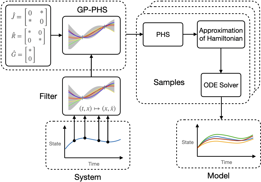
Figure 1. Gaussian Process port-Hamiltonian systems enable physically consistent predictions with uncertainty quantification.

By leveraging that GPs are closed under affine operations, the dynamics of a PHS is integrated into the GP by

\[ \begin{align} \dot{x}&\sim \mathcal{GP}({\hat G}(x\mid{\varphi}_G)u,k_{phs}(x,x^\prime)), \end{align} \]

(12)

where the new kernel function \( k_{phs}\) is given by

\[ \begin{align*} k_{phs}(x,x^\prime)&=\sigma_f^2\hat{J}_R(x\mid {\varphi}_J,{\varphi}_R)\Pi(x,x^\prime)\hat{J}_R^\top(x^\prime\mid {\varphi}_J,{\varphi}_R)\notag\\ \Pi_{i,j}(x,x^\prime) &= \frac{\partial }{\partial z_i \partial z_j}\exp(-\|z- z^\prime\|_{\Lambda}^2)\Big\vert_{z=x,z^\prime=x^\prime} \end{align*} \]

with the Hessian \( \Pi\) of the squared exponential kernel, see [66], and estimates \( \hat G,\hat{J}_R=\hat J-\hat R\) . Thus, the dynamics (12) describes a prior distribution over PHS. We start the training of the GP-PHS by using the collected dataset of timestamps \( \{t_i\}_{i=1}^N\) and noisy state observations with inputs \( \{\tilde x(t_i),{u}(t_i)\}_{i=1}^N\) of (6) in a filter to create a dataset consisting of pairs of states \( X=[x(t_1),…,x(t_N)]\) and state derivatives \( \dot{X}=[\dot{x}(t_1),…,\dot{x}(t_N)]\) . Then, the unknown (hyper)parameters \( \varphi=[\sigma_f,\Lambda,\varphi_G,\varphi_J,\varphi_R]\) can be optimized by minimizing the negative log marginal likelihood \( -\log \mathrm{p}(\dot{X}\vert \varphi,X)\sim\dot{X}_0^\top K_{phs}^{-1} \dot{X}_0+\log\vert K_{phs} \vert\) , with the mean-adjusted output data \( \dot{X}_0=[[\dot{x}(t_1)-\hat{G}{u}(t_1)]^\top,…,[\dot{x}(t_{N})-\hat{G}{u}(t_{N})]^\top]^\top\) . Once the GP model is trained, we can compute the posterior distribution using the joint distribution with mean-adjusted output data \( \dot{X}_0\) at a test states \( x^*\)

\[ \begin{align} \begin{bmatrix}\dot{X}_0\\ \dot{x} \end{bmatrix}=\mathcal{N}\left({0},\begin{bmatrix}K_{phs} & k_{phs}(X,x^*)\\ k_{phs}(X,x^*)^\top & k_{phs}(x^*,x^*)\end{bmatrix}\right)\notag. \\\end{align} \]

(13)

Analogously to the vanilla GP regression, the posterior distribution is then fully defined by the mean \( \mu\left(\dot{x}\mid\!x^{*}, D\right)\) and the variance \( \Sigma\left(\dot{x}\mid\!x^{*}, D\right)\) . Finally, we draw samples from the posterior distribution, where each sample represents a possible PHS given the data set \( D\) , and compute the solution of each sample using a standard ODE solver. The approach has been extended to enable physically consistent learning of switching systems [70] and PDE systems [71] with unknown dynamics, and has been applied to design robust, passivity-based controllers [72].

2.3.2 Uncertainty Quantification with Conformal Prediction in Physics-constrained Motion Prediction (PCMP)

To quantify prediction uncertainty in PCMP, we can employ conformalized quantile regression (CQR) [73, 74], which constructs statistically valid prediction regions. A scoring function \( s\) measures the deviation between predicted and observed states. Two novel tailored scoring functions are proposed in PCMP. In the {Rotated Rectangle Region} method, each predicted state is transformed into the robot’s local coordinate frame, aligned with its heading. The scoring function computes the deviation along the local \( x\) and \( y\) axes, preserving directional uncertainty. In the {Frenet Region} method, where map information is available, errors are defined in the Frenet frame, following the curve of the driving track, where progress along the centerline and lateral deviation are used. These robot-aware prediction regions improve interpretability and ensure that the uncertainty bounds respect road geometry.

Using the above scoring functions, the prediction region is constructed by the CQR method. The non-conformity score at each timestep is \( R_i = \max \{ q_\text{low} - s_i, s_i - q_\text{high} \}\) where \( q_\text{low}\) and \( q_\text{high}\) are empirical quantiles from a calibration set. The final prediction region at confidence level \( 1 - \delta\) is \( P_{t} = [q_\text{low} - E_{1-\delta}, \; q_\text{high} + E_{1-\delta}]\) where \( E_{1-\delta}\) is a quantile of the non-conformity scores. The true future state lies in \( P_t\) with at least \( 1 - \delta\) probability, even under multi-step predictions. As the result of uncertainty quantification, these prediction regions are used to ensure the (probabilistic) safety of risk-aware decision-making, such as autonomous robot control or driving algorithms.

3 Safe Learning for Control

Guaranteeing safety while learning or deploying learned components in control is crucial across various applications, ranging from autonomous driving to human-robot interaction. In such safety-critical domains, even minor control errors can lead to accidents; therefore, integrated safety measures are essential. As machine learning techniques are increasingly integrated into control systems, ensuring safety and stability remains a significant challenge. Unlike traditional controllers with well-defined behavior, learned components (e.g., neural network controllers or adaptive policies) can exhibit unpredictable actions if not properly constrained. This makes it vital to develop methods that ensure any learned behavior stays within safe bounds at all times.

In this section, we first explore how learning can be incorporated into model predictive control (MPC) while maintaining physical consistency and safety. We highlight recent advances in learning for MPC, including structured learning techniques and Bayesian optimization approaches that account for physical constraints during policy and parameter adaptation. Next, we briefly review (predictive) safety filters, which serve as modular safety layers, ensuring constraint satisfaction even when using uncertain learned models. Additionally, we review control barrier and Lyapunov function-based approaches that provide theoretical guarantees for stability and safety in learning-based control. We conclude by discussing Neural Lyapunov Control, which aims to jointly design a control policy and a corresponding Lyapunov stability certificate.

3.1 Learning-based Model Predictive Control and Predictive Safety Filters

MPC is based on the repeated solution of an optimal control problem (in continuous or discrete time), and the application of the first part of the optimal input before new state information becomes available [75, 76]. For simplicity of presentation, consider discrete-time dynamical systems given by

\[ \begin{equation} x_{k+1} = f(x_k, u_k). \end{equation} \]

(14)

Here \( x_k \in \mathbb{R}^{n_\text{x}}\) denote the system states, \( u_k \in \mathbb{R}^{n_\text{u}}\) are the system inputs, \( f: \mathbb{R}^{n_\text{x}} \times \mathbb{R}^{n_\text{u}} \to \mathbb{R}^{n_\text{x}}\) is the dynamics function, and \( k \in \mathbb{N}_0\) is the discrete time index.

At every discrete time index \( k\) and the measurement of the current state \( x_k\) , one solves the optimal control problem

\[ \begin{equation} \text{minimize}_{\mathbf{\hat{u}}_k } J = \left\{ \sum_{i=0}^{N-1} \ell({\hat x}_{i \mid k}, {\hat u}_{i \mid k}) + E({\hat x}_{N \mid k}) \right\} \end{equation} \]

(15.a)

\[ \begin{equation} \text{such that } \forall i \in \{0, 1, \dots, N-1\}: \notag \end{equation} \]

(15.b)

\[ \begin{equation} \hat x_{i+1\mid k} = \hat f(\hat x_{i\mid k}, \hat u_{i\mid k}),\hat x_{0 \mid k} = x_k, \end{equation} \]

(15.c)

\[ \begin{equation} \hat x_{i \mid k} \in \mathcal{X},{\hat u}_{i \mid k} \in \mathcal{U},\hat x_{N \mid k} \in \mathcal{E}. \end{equation} \]

(15.d)

Here, \( \hat{\cdot}_{i\mid k}\) denotes the model-based \( i\) -step ahead prediction at time index \( k\) . \( \hat{f}_ : \mathbb{R}^{n_\text{x}} \times \mathbb{R}^{n_\text{u}} \to \mathbb{R}^{n_\text{x}}, (x, u) \mapsto \hat{f}_\theta(x, u)\) is the prediction model. The length of the prediction horizon is \( N \in \mathbb{N}\) , \( N < \infty\) and \( \ell: \mathbb{R}^{n_\text{x}} \times \mathbb{R}^{n_\text{u}} \to \mathbb{R},\) and \( E : \mathbb{R}^{n_\text{x}} \to \mathbb{R},\) are the stage and terminal cost functions, respectively. The constraints (15.d) are comprised of the state, input, and terminal sets \( \mathcal{X}_\theta \subset \mathbb{R}^{n_\text{x}}\) , \( \mathcal{U} \subset \mathbb{R}^{n_\text{u}}\) , and \( \mathcal{E} \subset \mathbb{R}^{n_\text{x}}\) , respectively. Minimizing the cost over the control input sequence \( \mathbf{\hat{u}}_k(x_k)=[\hat u_{0 \mid k}(x_k),\dots,\hat u_{N-1 \mid k}(x_k; \theta)]\) results in the optimal input sequence \( \mathbf{\hat{u}}_k^*(x_k)\) , of which only the first element is applied to system (14). Subsequently, the optimal control problem (15) is solved again at all following time indices \( k\) . Consequently, the control policy is given by \( u_k = \hat u_{0 \mid k}^*(x_k)\) .

If the model perfectly captures the real system dynamics, stability and constraint satisfaction—ensuring safety—can be guaranteed, provided the problem is initially feasible and the cost function, along with the terminal cost, is properly designed [75]. However, in the presence of model uncertainty or external disturbances, robust, set-based, and stochastic MPC approaches have been developed to maintain stability and enforce constraints. While these methods enhance reliability under uncertainty, they often introduce conservatism, potentially limiting performance [77, 78, 79, 80, 81].

While robust and stochastic MPC approaches provide safety guarantees under uncertainty, they often lead to conservative behavior. This conservatism arises because these methods typically assume worst-case disturbances or use probabilistic bounds, resulting in overly cautious control actions that limit performance. Set-based approaches, such as tube-based MPC [81], ensure constraint satisfaction for all possible disturbances but can unnecessarily restrict the system’s capability. Similarly, scenario-based and stochastic MPC [78] formulations must balance constraint satisfaction probabilities with tractability, leading to suboptimal performance in many practical applications.

Learning-based techniques offer a promising path to reduce this conservatism [82, 62] by adjusting the model, cost function, and constraints based on measured data. However, integrating learning-based components introduces challenges in maintaining feasibility, stability, and robustness. Addressing these challenges has led to a growing focus on ensuring that the learned models and controllers respect physical constraints and stability criteria [83, 62, 84].

Basically, any component of the MPC formulation (15) can be learned, including the cost functions \( \ell\) , \( E\) [85, 86, 87], references and disturbances[88, 89] the constraints \( \mathcal{X}\) , \( \mathcal{U}\) [90, 91], or the system model \( \hat f\) , see [62] for a detailed discussion and classification. Furthermore, one can learn the MPC feedback law itself [92, 93, 94, 95, 96, 97, 98, 99] or utilize MPC as a safety layer/filter for learning-based controllers [83, 82]. Most of these approaches relay on suitably tailored robust predictive control formulations, to guarantee safety and stability, or an sampling based validation of the closed-loop properties.

3.1.1 Learning the Cost Function or Constraints via Differentiable MPC

A key challenge in safe learning for control is adapting the cost function or constraints in MPC to unknown or evolving system dynamics while maintaining stability and safety guarantees. The work on Differentiable MPC [87] provides a framework where both the cost function and constraints can be learned directly from data, enabling end-to-end training of control policies. This requires a slight modification of the MPC problem (15) by parametrizing the objective \( \ell({\hat x}_{i \mid k}, {\hat u}_{i \mid k}, \theta)\) and dynamics constraints \( \hat x_{i+1\mid k} = \hat f(\hat x_{i\mid k}, \hat u_{i\mid k}, \theta)\) with trainable parameters \( \theta\) .

In this approach, an MPC problem is formulated as a differentiable convex optimization layer [100, 101], where the cost function and system dynamics model parameters are learned jointly through backpropagation. Specifically, differentiable MPC incorporates a differentiable quadratic optimization solver that enables gradient-based updates of \( \theta\) . By leveraging automatic differentiation, the gradient of the MPC objective with respect to the learnable parameters can be computed as

\[ \begin{equation} \frac{d J}{d \theta} = \sum_{i=0}^{N-1} \frac{\partial \ell}{\partial \theta} + \sum_{i=0}^{N-1} \lambda_t \frac{\partial \hat f}{\partial \theta}, \end{equation} \]

(16)

where \( \lambda_t \) are the Lagrange multipliers associated with the dynamic system constraints.

An extension of this framework is learning components of a broad family of differentiable control policies [102]. Other notable extensions to this work, include differentiable robust MPC [103] to handle system uncertainties, or using reinforcement learning to tune differentiable MPC policies [104, 105, 106] for provably safe control. By integrating differentiable optimization with machine learning, this approach bridges the gap between traditional control theory and modern deep learning techniques, enabling real-time adaptive control in dynamic, uncertain environments.

3.1.2 Predictive Safety Filters (PSF)

PSF ensure safe operation in control systems by modifying control inputs in real time to prevent constraint violations. These filters use predictive models of system dynamics (14) that can be either physics- or learning-based to anticipate unsafe situations and minimally adjust control actions only when necessary, allowing the nominal controller to operate freely when safety is not at risk. They are particularly useful in learning-based control, where data-driven policies may lack formal guarantees of safety.

A predictive safety filter solves a constrained optimization problem at each time step

\[ \begin{align} \min_{u_t} & ~ \| u_t - u_t^\text{nom} \|^2 \\ \text{s.t.} & ~ x_{t+1} = f(x_t, u_t), \\ & ~ h(x_t, u_t) \geq 0, ~ \forall t. \\\end{align} \]

(17.a)

where \( u_t^\text{nom} \) is the nominal control input generated by an external policy (e.g., a reinforcement learning controller), and \( h(x_t, u_t) \geq 0 \) defines a safety constraint that must be satisfied at all times. This formulation ensures minimal deviation from the nominal control while enforcing safety.

An effective implementation of predictive safety filters is based on MPC [107], which predicts future states over a finite horizon and optimizes control adjustments to ensure safety. Unlike traditional MPC, which is designed for optimal performance, predictive safety filters focus purely on safety enforcement, allowing the primary controller to retain its autonomy whenever possible. This approach formulates the MPC safety filtering problem as a quadratic program (QP) that needs to be solved online to guarantee the stability of the closed-loop system [108]. Due to their stability guarantees based on MPC theory [109], predictive safety filters have been applied in safety-critical applications such as autonomous racing [110]. Extensions to MPC-based predictive safety filters include conformal prediction to provide uncertainty quantification [111], relaxed formulations with soft-constrained control barrier functions [7], extensions to nonlinear systems dynamics [112], or event-triggered mechanisms for reducing the computational requirements [113].

Despite their advantages, MPC-based safety filters require QP solvers capable of handling the online computation of constrained control adjustments. Recent advancements in fast quadratic programming solvers [114] have improved the scalability of these methods, enabling their application in complex, high-dimensional systems. By integrating predictive safety filters with learning-based controllers, it is possible to achieve both adaptability and formal safety guarantees, enhancing the robustness of real-world control systems.

3.2 Control Barrier and Control Lyapunov Functions

Lyapunov Functions (LF), Control Lyapunov Functions (CLFs), and Control Barrier Functions (CBFs) are fundamental tools in ensuring stability and safety in control systems, particularly when integrating learning-based or data-driven models with formal guarantees [4, 5, 6, 7]. Let’s assume a dynamical system in control affine form

\[ \begin{equation} \dot{x} = f(x) + g(x) u. \end{equation} \]

(18)

A CLF is used to ensure stability of (18) by providing a scalar function that decreases along system trajectories under an appropriate control input. Specifically, a continuously differentiable function \( V(x) \) is a CLF if there exist positive constants \( c_1, c_2 > 0 \) such that \( c_1 \| x \|^2 \leq V(x) \leq c_2 \| x \|^2, \forall x \in \mathbb{R}^n\) , and for all nonzero \( x \), there exists a control input \( u \) such that

\[ \begin{equation} \inf_{u} \left[ \frac{\partial V}{\partial x} (f(x) + g(x) u) \right] \leq -\alpha(V(x)), \end{equation} \]

(19)

for some positive class-\(\mathcal{K}\) function \( \alpha(\cdot) \). This condition ensures that an appropriate control input can always be found to drive the system towards equilibrium, guaranteeing asymptotic stability.

On the other hand, a CBF is designed to enforce safety constraints by ensuring that the system remains within a specified safe set. If a function \( h(x) \) defines the safe set as \( \{ x \mid h(x) \geq 0 \}\) , then a valid control input must satisfy

\[ \begin{equation} \sup_{u} \left[ \frac{\partial h}{\partial x} (f(x) + g(x) u) \right] \geq -\alpha(h(x)), \end{equation} \]

(20)

ensuring that trajectories do not exit the safe region. In practical implementations, CBFs and CLFs are often combined in a quadratic program framework to balance stability and safety objectives, particularly in real-time control of robotic systems, autonomous vehicles, and other safety-critical applications. These techniques are increasingly integrated with machine learning models to provide certifiable safety guarantees in data-driven controllers, ensuring that learned policies respect both stability and safety constraints in uncertain environments.

In the following two paragraphs, we provide two related examples for data-driven neural Lyapunov function candidates for stability verification of autonomous and closed-loop controlled dynamical systems with learning-based controllers.

3.2.1 Learning Neural Lyapunov Functions

The Lyapunov function (LF) can be interpreted as a scalar-valued function of potential energy stored in the system. LF are important notions in the control theory and stability theory of dynamical systems. For certain classes of ODEs, the existence of LF is a necessary and sufficient condition for stability. However, obtaining LF analytically for a general class of systems is not available, while existing computational methods, such as the Sum of Squares method [115], are intractable for larger systems. Approaches for learning neural LF candidates from dynamical system data [116, 117, 118, 119, 120, 121] presented a tractable alternative.

Let’s consider the problem of learning the LF that can be used to certify the stability of a dynamical system based on the observation of its trajectories. Specifically, lets assume autonomous system dynamics given by \( \dot{x} = f(x); \,\,\, x \in R^n \) , with available dataset of state observations \( X = [x^i_1, ..., x^i_N]\) , \( i = 1,...,m\) . Where \( N\) defines the length of the rollout, and \( m\) defines the number of sampled trajectories. The objective is to find a LF candidate \( V_{\theta}(x): R^n \to R; \,\,\, V_{\theta}(0) = 0; \,\,\, V_{\theta}(x) >0, \forall x \neq 0 \) , parametrized by \( {\theta}\) , that satisfies the discrere-time Lyapunov stability criterion \( V_{\theta}(x_{k+1}) - V_{\theta}(x_k) < 0\) for the given dataset of trajectories \( X\) .

We chose the neural LF candidate as presented in [118]. The architecture is based on the input convex neural network (ICNN) [46] followed by a positive-definite layer. The ICNN with \( L\) layers is defined as

\[ \begin{align} & z_1 = \sigma_0(W_0 x + b_0) \\ & z_{i+1} = \sigma_i(U_i z_i + W_i x + b_i), \,\,\, i \in \mathbb{N}_1^{L-1} \\ & g_{\theta}(x) = z_k \\\end{align} \]

(21.a)

Where \( W_i, b_i \) are real-valued weights and biases, respectively, while \( U_i\) are positive weights, and \( \sigma_i\) are convex, monotonically non-decreasing non-linear activations of the \( i\) -th layer. The trainable parameters of the ICNN architecture are given by \( \theta = \{ W_0, b_0, W_i, b_i, U_i \}, i \in \mathbb{N}_1^{L-1} \) . This ICNN layer guarantees that there are no local minima in the LF candidate \( V_{\theta}(x)\) . The ICNN is followed by a positive-definite layer

\[ \begin{equation} V_{\theta}(x) = \sigma_{k+1}(g_{\theta}(x) - g_{\theta}(0)) + \epsilon ||x||^2_2, \end{equation} \]

(22)

that acts as a coordinate transformation enforcing the condition \( V_{\theta}(0) = 0\) .

The general data-driven approach is to use stochastic gradient descent to optimize the parameters \( \theta\) of the neural LF candidate \( V_{\theta}(x)\) over the dataset of the state trajectories \( X\) using the physics-informed neural network (PINN) [122] approach of penalizing the expected risk of constraints violations given by the loss function

\[ \begin{equation} \mathcal{L}(X) = \sum_{i=1}^m \sum_{k=1}^{N-1} || \max \{0, V_{\theta}(x^i_{k+1}) - V_{\theta}(x^i_k)\} ||_2^2. \end{equation} \]

(23)

The disadvantage of the PINN approach with a soft-constrained loss function (23) is that it does not satisfy the Lyapunov stability criterion. To alleviate this issue in the context of system identification and learning-based controls, authors have proposed additional projection layers to correct the dynamics of the modeled system [118].

The open-source code demonstrating this tutorial example on a specific dynamical system can be found in the NeuroMANCER library [33].

3.2.2 Physics-informed Neural Lyapunov Lyapunov Control

Beyond learning a Lyapunov certificate for a given autonomous system, one can jointly design a control policy and its corresponding Lyapunov stability certificate. Some of the existing works on this topic include [123, 124, 125, 126, 127, 128].

Consider the nonlinear system \( \dot{x} = f(x, u)\) , where \( (x,u) \in \mathcal{D} \times \mathcal{U} \) is the state-control pair. The goal is to design or learn a control policy \( \pi_{\gamma}(\cdot) \) that stabilizes an equilibrium while optimizing a performance metric, such as maximizing the region of attraction (RoA), which serves as a robustness margin against uncertainties. A common learning-based approach parameterizes both the Lyapunov function \( V_\theta \) and controller \( \pi_{\gamma} \) using neural networks. Stability is enforced by minimizing the expected violation of Lyapunov conditions

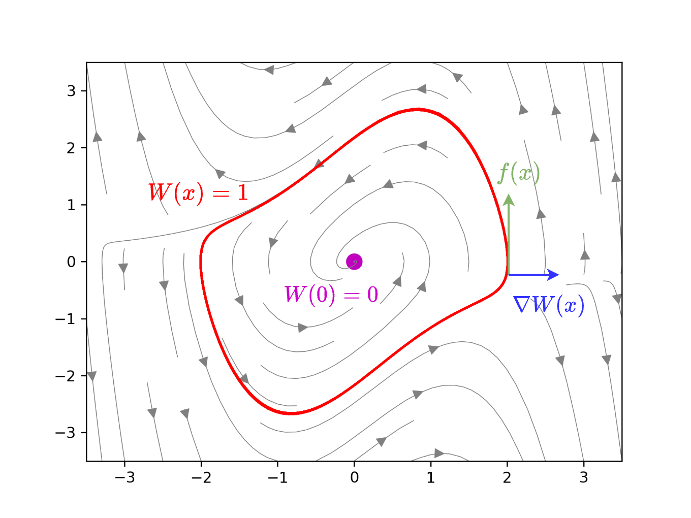
\[ \min_{\theta, \gamma} E_{x \sim \rho} \bigg[ V_\theta(0)^2 + (-V_\theta(x))_{+} + \big(\nabla_x V_\theta(x)^\top f(x, \pi_\gamma(x))\big)_{+} \bigg]. \]

However, this optimization can admit trivial solutions, such as \( V_{\theta}(x) = 0 \) for all \( x \in \mathcal{D} \). Regularizations such as \( ( \|x\|_2 - \alpha V_\theta(x) )^2\) can be used to encourage large RoAs [124], though poor choices may misalign the learned Lyapunov level sets with the true RoA. To address this, [129] proposes a physics-informed loss based on Zubov’s PDE, which directly captures the RoA. The PDE,

\[ \nabla W(x)^\top f(x,\pi_{\gamma}(x)) + \Psi(x)(1 - W(x)) = 0, \]

defines the Zubov function \( W(x) \in (0,1) \), with \( \Psi(x) \) as a positive definite function. Intuitively, this ensures that the Lie derivative of \( W \) is zero on the RoA boundary, precisely identifying the domain of attraction (see Figure 2 for an illustration).

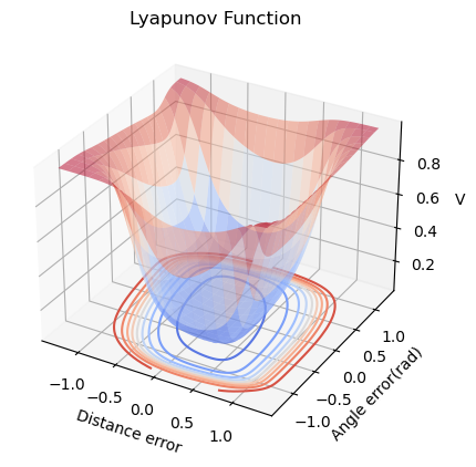
The level set {x : W(x)=1}) obtained by the Zubov PDE characterizes the boundary of the true DoA. — Figure 2. The level set \( {x : W(x)=1}\) obtained by the Zubov PDE characterizes the boundary of the true DoA.

Guided by Zubov’s PDE, the learned Lyapunov function is depicted in Figure 4. The verified region of attraction and the vector field of the learned controller are shown in Figure 5.

W_{}(x)) learned for bicycle tracking system — Figure 4. \( W_{\theta}(x)\) learned for bicycle tracking system

Verified DoA and vector field x = f(x, _(x))) — Figure 4. \( W_{\theta}(x)\) learned for bicycle tracking system

4 Safety Verification Methods

Safety verification methods aim to formally or empirically certify that a system operates within predefined safety constraints under all possible disturbances and uncertainties. These methods broadly fall into three categories: reachability analysis methods [130, 131], constrained optimization-based methods [132, 133], and simulation and sampling-based approaches [134, 135, 136]. Reachability analysis constructs forward or backward reachable sets to determine whether unsafe states can be reached from an initial condition, providing rigorous guarantees of safety but often facing scalability challenges in high-dimensional systems. Constrained optimization-based approaches formulate safety verification as an optimization problem where system constraints, safety conditions, and physical limitations are explicitly incorporated. The goal is to determine whether a system can violate predefined safety conditions by solving an optimization problem that seeks counterexamples or guarantees safe operation. Simulation and sampling-based approaches, including Monte Carlo simulations and probabilistic verification, offer a scalable alternative by empirically evaluating system behavior over a large number of sampled scenarios, often at the cost of completeness. Together, these techniques form a diverse toolkit for verifying and enforcing safety in complex, uncertain environments, striking a balance between computational feasibility and formal guarantees.

4.1 Reachability Analysis Methods

In safety-critical systems, reachable set analysis determines all possible states a dynamical system can reach from a given set of initial conditions and inputs. Safety verification often requires ensuring that the reachable set never intersects unsafe states. However, computing exact reachable sets is generally intractable, except in special cases. Existing approaches for reachability analysis fall into two broad categories: set propagation techniques and Hamilton-Jacobi reachability.

4.1.1 Set Propagation Techniques

Given the system \( x^{k+1} = f(x^k), x^0 \in \mathcal{X}^0\) , where \(\mathcal{X}^0\) is a bounded set of initial conditions, the reachable set at time \( k+1 \) is

\[ \mathcal{X}^{k+1} = f(\mathcal{X}^k) = \{f(x) \mid x \in \mathcal{X}^k\}. \]

Since exact computation is generally intractable, reachable sets are typically over-approximated using {template sets} \((\bar{\mathcal{X}}_k)_{k\geq 0}\), where \(\bar{\mathcal{X}}^0 = \mathcal{X}^0\) and each step ensures \( f(\bar{\mathcal{X}}^k) \subseteq \bar{\mathcal{X}}^{k+1} \) via a {set propagation algorithm} often relying on convex relaxations. If these sets avoid unsafe regions, safety is guaranteed.

Convex relaxations improve computational tractability but introduce conservatism, particularly when the actual reachable set is nonconvex or irregularly shaped. The resulting over-approximation errors can accumulate over time—a phenomenon known as the wrapping effect [137]—leading to increasingly conservative bounds.

Conservatism due to nonconvexity can be reduced by employing tighter convex relaxations that aim to approximate the convex hull of the reachable set, partitioning input sets to refine the resolution or selecting templates that better match the geometry of the reachable set. The choice of template sets, such as ellipsoids or polyhedra, significantly impacts accuracy. A poor match between the template shape and the true reachable set leads to shape mismatch error, even with tight convex relaxations.

Dynamic templates can help mitigate these errors by adapting to the geometry of \( f\) . Oriented hyperrectangles, obtained via principal component analysis (PCA) on sampled trajectories [138], are computationally efficient but can still be overly conservative. More sophisticated methods exist, such as those in [139], which solve convex optimization problems to determine template polytope directions, or in [140], where a first-order Taylor approximation of \( f\) (assuming differentiability) is used to guide template adaptation. A more recent approach in [141] leverages a ReLU network to dynamically adjust polytopic templates, offering a data-driven way to better approximate the reachable set.

4.1.2 Hamilton Jacobi Reachability

Hamilton–Jacobi (HJ) reachability is a powerful method for computing reachable sets in dynamical systems by leveraging optimal control theory and level-set methods. It formulates safety verification as a Hamilton–Jacobi–Isaacs partial differential equation (HJI-PDE) [142], where the value function \( V(x,t)\) defines the boundary of the reachable set as its zero level-set. By solving this PDE forward or backward in time, HJ reachability provides precise characterizations of system behaviors, accounting for nonlinear dynamics and adversarial disturbances. This rigorous approach makes HJ reachability a gold standard in safety verification, particularly for applications requiring guaranteed safety under worst-case uncertainties. However, despite its accuracy, the method suffers from the curse of dimensionality, as solving the HJI-PDE becomes computationally intractable for high-dimensional systems, limiting its scalability to complex real-world applications. Recent advancements, including neural approximations [143, 144, 145] and decomposition techniques [146, 147], aim to mitigate these limitations and extend the applicability of HJ reachability to large-scale dynamical systems.

4.2 Constrained Optimization-based Methods

Many verification problems can be posed as proving the positivity of a function over a specified domain \( \min_{x\in X} f(x) \ge 0\) . Common examples include demonstrating the existence of a Lyapunov function, computing an invariant region in which constraints are satisfied, and certifying a maximum error for an approximate control computation over a region of interest. Such problems have long been studied in the control literature, and the ability to solve these challenging problems depends very heavily on the properties of the system, control law and property being verified (the function \( f\) ), as well as the structure of the domain \( X\) .

4.2.1 Verificaiton via Mixed-integer Linear Programming

One approach that can be used for a number of important verification problems is to map the positivity verification problem onto a mixed-integer linear programming structure (MILP), which is then solvable to global optimality using standard tools, thereby providing rigorous guarantees for a variety of physical properties, as well as safety and stability. Problems that have such a mapping are dubbed ‘MILP-representable verification problems’ [148].

At the core of these approaches is the concept of MILP-representable functions. Such functions \( \psi: X \rightarrow U \) have graphs that can be exactly characterized by linear inequalities and equalities involving continuous and binary variables. Formally, a function \( \psi : \mathbb{R}^n \mapsto \mathbb{R}^m \) is called MILP-representable if there exists a polyhedral set \( P \subseteq \mathbb{R}^{n+m+c+b} \) such that

\[ \begin{equation} (x,u) \in \text{gr}(\psi) \Leftrightarrow \exists p \in \mathbb{R}^c, \beta \in \{0,1\}^b: (x,u,p,\beta) \in P. \end{equation} \]

(24)

One can show that the set of MILP-representable functions are dense in the family of continuous functions on a compact domain with respect to the supremum norm, and that the composition of MILP-representable functions is also MILP-representable. This formulation allows a diverse set of systems and controllers to be modeled exactly, including piecewise-affine systems, the optimal solution map of a parametric quadratic program (such as MPC), or controllers defined by ReLU NNs.

To illustrate, we take the simple example of a controller that computes its input via a fully-connected deep neural network \( \phi : \mathbb{R}^n \rightarrow \mathbb{R}\) , which is a composition of ReLU layers \( \phi = \phi_l \circ \phi_{l-1} \circ \dots \circ \phi_0\) , where \( \phi_i : \mathbb{R}^{n_i} \rightarrow \mathbb{R}^{m_i}\) . The ReLU function is defined as

\[ \begin{align*} \phi_i(z_{i-1}) = ReLU(z_{i-1}) = \max(0, W_iz_{i-1}+b_i), \end{align*} \]

for weight matrix \( W_i\) and bias vector \( b_i\) . We define the polyhedron \( P_i\) as

\[ \begin{align*} P_i = \left\{ (z_{i-1},z_i,p,\beta_i\left. \begin{aligned} |z_i - (W_iz_{i-1}+b_i)| &\le M(1-\beta_i)\\ 0 \le z_i &\le M\beta_i \end{aligned} \right.\right\} \end{align*} \]

where \( M\) is a sufficiently large positive constant. We can see that \( z_i = \phi_i(z_{i-1})\) if and only if there exists a \( \beta_i \in \{0,1\}^{m_i}\) such that \( (z_{i-1}, z_i, p, \beta_i) \in P_i\) .

Suppose now that we have the simple verification goal of computing the maximum value that the controller may take for any state in the polyhedral set \( X\) . i.e., we want to solve the verification problem \( \max_{x \in X}\phi(x)\) . Because the controller is MILP-representable, this problem can be written as a standard MILP (25).

\[ \begin{align} \max_{x\in X}u\\ \text{s.t.} \begin{aligned}[t] (x, z_1, p_1, \beta_1) &\in P_1\\ (z_{i-1}, z_i, p_i, \beta_i) &\in P_i~ \forall i = 2\dots,l-1\\ (z_{l-1}, u, p_l, \beta_l) &\in P_l\\ \beta_i &\in {0,1}^{n_i}~ \forall i = 1\dots,l \end{aligned} \\\end{align} \]

(25.a)

While we have followed the formalism introduced in [148] here, there are several variations of this concept in the literature. [149] captures neural-network controllers in MILP form, before doing a reachability analysis, while [150, 151] represent PWA Lyapunov functions in a similar formalism while executing a learner/verifier pattern. [152] combines a MILP representation with a Lipschitz bound to conservatively compute a bound on the approximation error of a neural network. In addition, there are a number of papers studying similar representations in the machine learning community for various neural network verification problems unrelated to control.

4.3 Simulation and Sampling-based Methods

Simulation or sampling-based methods provide a simple and scalable alternative for verification tasks for complex dynamical systems with possibly unknown components. Due to their flexibility and practical performance in high-dimensional systems, they have gained popularity for approximating reachable sets [134, 153, 154, 155, 156, 157], invariant sets [135, 158, 159], or regions of attraction [136, 160]. In this section, we briefly overview its main components and the types of guarantees that one can achieve.

4.3.1 Sampling-based Reachability Analysis

In sampling-based reachability analysis, one is given a set \( \mathcal{X}\) and map \( f:\mathbb{R}^m\rightarrow\mathbb{R}^n\) , with the goal of approximating the set

\[ \begin{equation} \mathcal{Y}=f(\mathcal{X})=\{f(x):x\in\mathcal{X}\} \end{equation} \]

(26)

that is reached from \( \mathcal{X}\) using samples. Methods proposed in this context often consider the following elements:

A distribution \( \mathbb{P}_\mathcal{X}\) to sample points from \( \mathcal{X}\) .
A number \( N\) of i.i.d. samples \( \{(x_i, y_i = f(x_i))\}_{i=1}^N\) .
A parameter \( \epsilon\) quantifying conservativeness.
A hypothesis class \( \mathcal{H}\subset 2^{\mathbb{R}^n}\) of candidates set \( \hat{\mathcal{Y}}\) .

Given these elements, the role of sampling-based algorithms is to construct a set-valued map \( \hat{\mathcal{Y}}_\epsilon^N\) that maps the samples to an estimated set \( \hat{\mathcal{Y}} \in \mathcal{H}\) :

\[ \hat{\mathcal{Y}}_\epsilon^N:\{y_i\}_{i=1}^N \mapsto \hat{\mathcal{Y}}\in\mathcal{H}. \]

The choice of these elements naturally determines the outcome of this process, its computational complexity, and associated guarantees.

Choice of \( \mathcal{Y}_\epsilon^N\) and \( \mathcal{H}\) : In general, the selection of the hypothesis class \( \mathcal{H}\) , and as a result, the implementation of \( \mathcal{Y}_\epsilon^N\) could be as simple as computing a union balls \( \epsilon\) -padded points or normed balls [161, 162, 134, 156], e.g., \( \hat{\mathcal{Y}}_\epsilon^N = \{y_i\}_{i=1}^{N}\oplus B_\epsilon, \) its convex hull, i.e., \( \hat{\mathcal{Y}}_\epsilon^N = \mathrm{conv}\left(\{y_i\}_{i=1}^{N}\right)\oplus B_\epsilon\) [153, 154], or given by the \( \epsilon\) -sublevel set of a neural function approximation \( \hat{\mathcal{Y}}_\epsilon^N = \{y: V_\theta(y)\leq \epsilon\}\) [163], where the function \( V_\theta\) is trained using the samples. As a result, the complexity of computing the approximation can vary significantly.

Distribution \( \mathbb{P}_\mathcal{X}\) : The sampling distribution \( \mathbb{P}_\mathcal{X}\) is often a design parameter. Simple yet effective algorithms often choose a fix \( \mathbb{P}_\mathcal{X}\) , e.g., uniform, whose support covers \( \mathcal{X}\) or its boundary \( \partial\mathcal{X}\) . Alternatively, adaptive sampling approaches, e.g., using active learning [135], can be further leveraged to improve sample efficiency.

Formal Guarantees: Finally, guarantees on the validity and accuracy of the verification process can be given for different choices of \( N\) , \( \epsilon\) , and \( \mathcal{H}\) . These can be succinctly expressed using some notion of set distance \( d(P, Q)\) . A common example is the Hausdorff distance

\[ d_H(P, Q)=\max\{\,\adjustlimits\sup_{x\in P} \inf_{y\in Q}d(x,y),\; \adjustlimits\sup_{y\in Q} \inf_{x\in P}d(x,y)\,\}. \]

Alternatively, in some cases, other accuracy metrics are considered, e.g., \( d_\mathbb{P_\mathcal{X}}(\hat{\mathcal{Y}}_\epsilon^N, \mathcal{Y}) = \mathbb{P}_\mathcal{X}\left(\hat{\mathcal{Y}}_\epsilon^N\cap \mathcal{Y}\right)\) , although they struggle to capture the outer level of mismatch \( \hat{\mathcal{Y}}_\epsilon^N\) and \( \mathcal{Y}\) [157].

Almost Sure Guarantees: Taking \( N\) to infinity leads to

\[ \begin{equation} \lim_{N\rightarrow\infty} d_H(\hat{\mathcal{Y}}_\epsilon^N, \Pi_\mathcal{H}(\mathcal{Y})) \leq \epsilon ~ \text{a.s.} \end{equation} \]

(27)

where \( \Pi_\mathcal{H}(\mathcal{Y})\) is the best approximation of \( \mathcal{Y}\) within \( \mathcal{H}\) , e.g., \( \Pi_{\mathcal{H}}(\mathcal{Y}) = \mathrm{conv}(\mathcal{Y})\) for convex hull approximations. When \( \epsilon=0\) , this leads to consistent estimates [153].

High-probability Guarantees: For sufficiently large \( N\) , e.g., \( N \geq \Omega\left(\mathrm{poly}\left(\frac{1}{\epsilon}\right)\mathrm{polylog}\left(\frac{1}{\delta}\right)\right)\) , the condition (27) often reduces to guaranteeing

\[ \begin{equation} d_H(\hat{\mathcal{Y}}_\epsilon^N, \Pi_\mathcal{H}(\mathcal{Y})) \leq \epsilon \end{equation} \]

(28)

with probability \( 1-\delta\) [154], provided some additional assumption is considered on \( f\) , e.g., Lipschitz. We finalize highlighting that depending \( \mathcal{H}\) and the value of \( \epsilon\) , the corresponding \( \hat{\mathcal{Y}}_\epsilon^N\) , can also be guaranteed to either an inner approximation, for \( \epsilon=0\) , or outer approximation, for \( \epsilon>0\) and \( N\) large.

4.3.2 Sampling-based Estimation of Invariant Sets

Invariant sets, i.e., sets that keep trajectories within a specified region, can be similarly estimated via iterative sampling strategies similar to the ones described above. We briefly discuss here the main differences. In this setting, given a domain \( \mathcal{X}\) , we are interested in identifying set \( \mathcal{I}\subseteq \mathcal{X}\) , with the properties that trajectories \( x(t)\) satisfying

\[ \begin{equation} x(0)\in \mathcal{I}\implies x(t)\in \mathcal{I},~ \forall t\geq0. \end{equation} \]

(29)

Similarly to the reachability setting, one analogously defines \( \mathbb{P}_\mathcal{X}\) , number of samples inside and outside \( \mathcal{I}\) , \( N_i\) and \( N_o\) with \( N=N_i+N_o\) , a conservativeness parameter \( \epsilon\) , and a hypothesis class \( \mathcal{H}\) , and set estimate \( \hat{\mathcal{I}}_\epsilon^N\) . In particular, similar hypothesis classes \( \mathcal{H}\) are considered, including unions of balls [136], sub-level sets of neural function approximations [135, 160], or biased versions of nearest neighbors [158]. However, there are key notable differences in this setting that we highlight next.

Circular dependence of \( \hat{\mathcal{I}}_\epsilon^N\) : Given some \( x\in\mathcal{X}\) , checking condition (29) requires knowledge of \( \mathcal{I}\) , yet building an estimate \( \hat{\mathcal{I}}_\epsilon^N\) requires the identification of point \( x_i\in\mathcal{I}\) and \( x_o\not\in\mathcal{I}\) . This is usually circumvented by constructing implicit oracles of the condition \( \mathcal{O}(x) = \mathbb{1}_{\{x\in\mathcal{Y}\}}\) checking implicit invariance conditions such as convergence to a small ball around a stable equilibrium [135], finding a time \( t^*\) s.t. if \( x(t^*)\in\mathcal{X}\) , then \( x(t)\in\mathcal{X}\) \( \forall t\geq t^*\) [158], or checking a recurrence condition on \( \hat{\mathcal{I}}_\epsilon^N\) , [136], that guarantees the inclusion \( \hat{\mathcal{I}}_\epsilon^N\subseteq \mathcal{I}\) .

Non-uniqueness: The number of invariant sets within \( \mathcal{X}\) may be uncountable, thus introducing a level of indeterminism that makes the problem more challenging and algorithms more difficult to converge. This indeterminism is often overcome by targeting invariant sets that are maximal in some sense, like domains of attractions of stable equilibrium points [136, 160].

Formal Guarantees: Finally, we highlight that the type guarantees focus on quantifying the fraction of the volume of \( \hat{\mathcal{I}}_\epsilon^N\) that is invariant, e.g., stating that with probability \( 1-\delta\) , \( d_{\mathbb{P}_\mathcal{X}}(\hat{\mathcal{I}}_\epsilon^N,\mathcal{I})=\mathbb{P}_\mathcal{X}(\hat{\mathcal{I}}_\epsilon^N\cap\mathcal{I})\leq \epsilon\) as in [158]. However, it is guaranteeing \( \hat{\mathcal{I}}_\epsilon^N\) being invariant (with high probability) is generally difficult. At best, guarantees of the form \( \hat{\mathcal{I}}_\epsilon^N\subset \mathcal{I}\) with high probability, or a.s. in the limit \( N\rightarrow\infty\) are obtained in practice [136].

5 Challenges and Opportunities

The integration of safe physics-informed machine learning (PIML) in dynamical systems and control presents several challenges and opportunities.

A fundamental issue in uncertainty quantification (UQ) is the reliable estimation of uncertainties in learned models and controllers. Traditional machine learning techniques, such as Gaussian processes and Bayesian neural networks, provide probabilistic uncertainty estimates, but translating these estimates into actionable safety constraints remains challenging. Recent advancements in conformal prediction, probabilistic reachability, and risk-aware optimization offer promising directions for bridging this gap. Future work should focus on integrating these UQ techniques into real-time safety mechanisms such as predictive safety filters or coltrol barrier functions.

Another significant challenge is the trade-off between conservatism and performance in safe learning-based controllers. Robust and stochastic model predictive control (MPC) formulations, while effective in enforcing safety, often introduce excessive conservatism, leading to suboptimal performance. Learning-based methods such as differentiable MPC have the potential to reduce this conservatism by dynamically adapting constraints, cost functions, and disturbance models based on observed data. However, ensuring stability, feasibility, robustness, and online computational tractability while incorporating learned components for nonlinear systems remains an open question. Opportunities exist in developing novel adaptive safety filters and robust learning frameworks that dynamically adjust based on real-time uncertainty quantification, as well as novel offline pre-training mechanisms and event triggering mechanisms for reducing online computational loads.

Another major challenge is the safe exploration problem in reinforcement learning (RL) and adaptive control. Learning-based control policies often require exploration to improve performance, yet unrestricted exploration may lead to safety violations. While approaches such as control barrier functions (CBFs), Lyapunov-based stability certificates, and predictive safety filters (PSFs) provide mechanisms for enforcing safety, they can overly constrain learning, limiting policy improvement. A key research opportunity lies in developing efficient RL exploration strategies that balance safety with learning efficiency, potentially leveraging safe Bayesian optimization, risk-sensitive RL, and constrained offline policy optimization methods.

One of the primary challenges lies in the scalability of safe learning methods. Many existing approaches, such as Hamilton–Jacobi reachability analysis and Mixed-integer programming based safety verification, suffer from the curse of dimensionality, making their application to high-dimensional systems computationally infeasible. Although decomposition techniques and neural approximations have been proposed, ensuring both accuracy and efficiency remains a critical open problem. Developing scalable safety verification techniques that balance computational feasibility with rigorous safety guarantees is an essential direction for future research.

From a broader perspective, there is a need for unified frameworks that integrate multiple safety mechanisms. Current approaches often treat safe learning, safety verification, and robust control as separate problems. A more holistic approach would involve the co-design of learning algorithms, verification techniques, and real-time control strategies, ensuring that learned policies inherently satisfy safety and stability constraints. Such frameworks could leverage advances in differentiable optimization, neural-symbolic reasoning, and hybrid machine learning-control architectures to create adaptable and certifiably safe controllers.

Finally, the real-world deployment of safe PIML still presents several challenges related to robustness, interpretability, and trustworthiness. While theoretical guarantees provide confidence in controlled settings, real-world systems exhibit uncertainties that are difficult to model precisely. Bridging the gap between theory and practice requires further research in hardware-in-the-loop safety validation, domain adaptation, and human-in-the-loop safety monitoring. Opportunities exist in creating benchmarks, standardized evaluation metrics, and open-source safety tools to facilitate broader adoption of safe learning-based control methods in real-world applications.

6 Conclusions

Safe learning for dynamical systems presents a promising pathway for enabling high-performance decision-making and control for a wide range of safety-critical applications. By integrating learning-based approaches with formal safety verification and robust control principles, it is possible to achieve adaptive and certifiably safe autonomous systems. However, several practical challenges remain, including the scalability of safety verification methods, reliable uncertainty quantification, and robust deployment in uncertain and faulty real-world scenarios. Addressing these challenges requires advancements in real-time safety filtering, risk-aware and constrained machine learning, and unified frameworks that systematically combines learning, verification, and control. The future of safe learning lies in developing scalable, interpretable, and provably safe methodologies that bridge the gap between theory and real-world deployment, ensuring reliable operation in safety-critical applications such as energy systems, critical infrastructure, robotics, autonomous driving, and industrial automation.

References

[1] T. X. Nghiem, J. Drgoňa, C. Jones, Z. Nagy, R. Schwan, B. Dey, A. Chakrabarty, S. Di Cairano, J. A. Paulson, A. Carron, M. N. Zeilinger, W. Shaw Cortez, and D. L. Vrabie, “Physics-informed machine learning for modeling and control of dynamical systems,'' in 2023 American Control Conference (ACC), 2023, pp. 3735–3750.

[2] G. Karniadakis, I. Kevrekidis, L. Lu, P. Perdikaris, S. Wang, and L. Yang, “Physics-informed machine learning'', Nature Reviews Physics, vol. 3, no. 6, pp. 422–440, Jun. 2021, publisher Copyright: © 2021, Springer Nature Limited.

[3] J. Thiyagalingam, M. A. Shankar, G. Fox, and T. A. J. G. Hey, “Scientific machine learning benchmarks,'' Nature Reviews Physics, vol. 4, pp. 413 – 420, 2021. [Online]. Available: https://api.semanticscholar.org/CorpusID:239768180

[4] C. Dawson, S. Gao, and C. Fan, “Safe control with learned certificates: A survey of neural Lyapunov, barrier, and contraction methods for robotics and control,'' IEEE Transactions on Robotics, vol. 39, no. 3, pp. 1749–1767, 2023.

[5] L. Brunke, M. Greeff, A. W. Hall, Z. Yuan, S. Zhou, J. Panerati, and A. P. Schoellig, “Safe learning in robotics: From learning-based control to safe reinforcement learning,'' Annual Review of Control, Robotics, and Autonomous Systems, vol. 5, no. Volume 5, 2022, pp. 411–444, 2022. [Online]. Available: https://www.annualreviews.org/content/journals/10.1146/annurev-control-042920-020211

[6] S. Wang and S. Wen, “Safe control against uncertainty: A comprehensive review of control barrier function strategies,'' IEEE Systems, Man, and Cybernetics Magazine, vol. 11, no. 1, pp. 34–47, 2025.

[7] K. P. Wabersich, A. J. Taylor, J. J. Choi, K. Sreenath, C. J. Tomlin, A. D. Ames, and M. N. Zeilinger, “Data-driven safety filters: Hamilton-jacobi reachability, control barrier functions, and predictive methods for uncertain systems,'' IEEE Control Systems Magazine, vol. 43, no. 5, pp. 137–177, 2023.

[8] J. H. Tu, C. W. Rowley, D. M. Luchtenburg, S. L. Brunton, and J. N. Kutz, “On dynamic mode decomposition: Theory and applications,'' pp. 391–421, 2014. [Online]. Available: https://www.aimsciences.org/article/id/1dfebc20-876d-4da7-8034-7cd3c7ae1161

[9] R. T. Q. Chen, Y. Rubanova, J. Bettencourt, and D. Duvenaud, “Neural ordinary differential equations,'' in Proceedings of the 32nd International Conference on Neural Information Processing Systems, ser. NIPS'18. 1em plus 0.5em minus 0.4em Red Hook, NY, USA: Curran Associates Inc., 2018, p. 6572–6583.

[10] C. Legaard, T. Schranz, G. Schweiger, J. Drgoňa, B. Falay, C. Gomes, A. Iosifidis, M. Abkar, and P. Larsen, “Constructing neural network based models for simulating dynamical systems,'' ACM Comput. Surv., vol. 55, no. 11, Feb. 2023. [Online]. Available: https://doi.org/10.1145/3567591

[11] D. Gedon, N. Wahlström, T. B. Schön, and L. Ljung, “Deep state space models for nonlinear system identification⁎⁎this research was partially supported by the wallenberg ai, autonomous systems and software program (wasp) funded by knut and alice wallenberg foundation and the swedish research council, contracts 2016-06079 and 2019-04956.'' IFAC-PapersOnLine, vol. 54, no. 7, pp. 481–486, 2021, 19th IFAC Symposium on System Identification SYSID 2021. [Online]. Available: https://www.sciencedirect.com/science/article/pii/S2405896321011800

[12] D. Masti and A. Bemporad, “Learning nonlinear state-space models using deep autoencoders,'' in 2018 IEEE Conference on Decision and Control (CDC), 2018, pp. 3862–3867.

[13] S. L. Brunton, J. L. Proctor, and J. N. Kutz, “Discovering governing equations from data by sparse identification of nonlinear dynamical systems,'' Proceedings of the National Academy of Sciences, vol. 113, no. 15, pp. 3932–3937, 2016. [Online]. Available: https://www.pnas.org/doi/abs/10.1073/pnas.1517384113

[14] S. L. Brunton and J. N. Kutz, Data-Driven Science and Engineering: Machine Learning, Dynamical Systems, and Control, 2nd ed. 1em plus 0.5em minus 0.4em Cambridge University Press, 2022.

[15] J.-C. Loiseau and S. L. Brunton, “Constrained sparse Galerkin regression,'' Journal of Fluid Mechanics, vol. 838, pp. 42–67, 2018.

[16] Alan A Kaptanoglu and Jared L Callaham and Christopher J Hansen and Aleksandr Aravkin and Steven L Brunton Promoting global stability in data-driven models of quadratic nonlinear dynamics Physical Review Fluids 2021 6 094401

[17] M. Schlegel and B. R. Noack, “On long-term boundedness of galerkin models,'' Journal of Fluid Mechanics, vol. 765, pp. 325–352, 2015.

[18] T. Askham and J. N. Kutz, “Variable projection methods for an optimized dynamic mode decomposition,'' SIAM Journal on Applied Dynamical Systems, vol. 17, no. 1, pp. 380–416, 2018.

[19] Peter J Baddoo and Benjamin Herrmann and Beverley J McKeon and J Nathan Kutz and Steven L Brunton Physics-informed dynamic mode decomposition Proceedings of the Royal Society A 2023 479 2271 20220576

[20] B. Lusch, J. N. Kutz, and S. L. Brunton, “Deep learning for universal linear embeddings of nonlinear dynamics,'' Nature Communications, vol. 9, no. 1, p. 4950, Nov. 2018.

[21] E. Yeung, S. Kundu, and N. Hodas, “Learning deep neural network representations for Koopman operators of nonlinear dynamical systems,'' in 2019 American Control Conference (ACC), 2019, pp. 4832–4839.

[22] N. Takeishi, Y. Kawahara, and T. Yairi, “Learning Koopman invariant subspaces for dynamic mode decomposition,'' in Advances in Neural Information Processing Systems, I. Guyon, U. V. Luxburg, S. Bengio, H. Wallach, R. Fergus, S. Vishwanathan, and R. Garnett, Eds., vol. 30. 1em plus 0.5em minus 0.4em Curran Associates, Inc., 2017. [Online]. Available: https://proceedings.neurips.cc/paper_files/paper/2017/file/3a835d3215755c435ef4fe9965a3f2a0-Paper.pdf

[23] H. Shi and M. Q.-H. Meng, “Deep Koopman operator with control for nonlinear systems,'' IEEE Robotics and Automation Letters, vol. 7, no. 3, pp. 7700–7707, 2022.

[24] Y. Han, W. Hao, and U. Vaidya, “Deep learning of Koopman representation for control,'' in 2020 59th IEEE Conference on Decision and Control (CDC), 2020, pp. 1890–1895.

[25] E. Kaiser, J. N. Kutz, and S. L. Brunton, “Data-driven discovery of Koopman eigenfunctions for control,'' Machine Learning: Science and Technology, vol. 2, 2017. [Online]. Available: https://api.semanticscholar.org/CorpusID:49216843

[26] M. Han, J. Euler-Rolle, and R. K. Katzschmann, “DeSKO: Stability-assured robust control with a deep stochastic Koopman operator,'' in International Conference on Learning Representations, 2022. [Online]. Available: https://openreview.net/forum?id=hniLRD_XCA

[27] G. Mamakoukas, I. Abraham, and T. D. Murphey, “Learning stable models for prediction and control,'' IEEE Transactions on Robotics, vol. 39, no. 3, pp. 2255–2275, 2023.

[28] Petar Bevanda and Max Beier and Sebastian Kerz and Armin Lederer and Stefan Sosnowski and Sandra Hirche Diffeomorphically Learning Stable Koopman Operators 2022

[29] J. Drgoňa, A. Tuor, S. Vasisht, and D. Vrabie, “Dissipative deep neural dynamical systems,'' IEEE Open Journal of Control Systems, vol. 1, pp. 100–112, 2022.

[30] E. Skomski, S. Vasisht, C. Wight, A. Tuor, J. Drgoňa, and D. Vrabie, “Constrained block nonlinear neural dynamical models,'' in 2021 American Control Conference (ACC), 2021, pp. 3993–4000.

[31] J. Drgona, S. Mukherjee, J. Zhang, F. Liu, and M. Halappanavar, “On the stochastic stability of deep markov models,'' in Advances in Neural Information Processing Systems, M. Ranzato, A. Beygelzimer, Y. Dauphin, P. Liang, and J. W. Vaughan, Eds., vol. 34. 1em plus 0.5em minus 0.4em Curran Associates, Inc., 2021, pp. 24 033–24 047. [Online]. Available: https://proceedings.neurips.cc/paper_files/paper/2021/file/c9dd73f5cb96486f5e1e0680e841a550-Paper.pdf

[32] Jiong Zhang and Qi Lei and Inderjit S. Dhillon Stabilizing Gradients for Deep Neural Networks via Efficient SVD Parameterization 2018

[33] J. Drgona, A. Tuor, J. Koch, M. Shapiro, B. Jacob, and D. Vrabie, “NeuroMANCER: Neural Modules with Adaptive Nonlinear Constraints and Efficient Regularizations,'' 2023. [Online]. Available: https://github.com/pnnl/neuromancer

[34] T. Duong, A. Altawaitan, J. Stanley, and N. Atanasov, “Port-Hamiltonian Neural ODE Networks on Lie Groups for Robot Dynamics Learning and Control,'' IEEE Transactions on Robotics, vol. 40, pp. 3695–3715, 2024.

[35] S. Fiaz, D. Zonetti, R. Ortega, J. M. A. Scherpen, and A. J. van der Schaft, “A port-Hamiltonian approach to power network modeling and analysis,'' European Journal of Control, vol. 19, no. 6, pp. 477–485, Dec. 2013.

[36] K. Rath, C. G. Albert, B. Bischl, and U. von Toussaint, “Symplectic Gaussian process regression of maps in Hamiltonian systems,'' Chaos: An Interdisciplinary Journal of Nonlinear Science, vol. 31, no. 5, p. 053121, May 2021.

[37] C. Neary and U. Topcu, “Compositional Learning of Dynamical System Models Using Port-Hamiltonian Neural Networks,'' in Proceedings of The 5th Annual Learning for Dynamics and Control Conference. 1em plus 0.5em minus 0.4em PMLR, Jun. 2023, pp. 679–691.

[38] J. Rettberg, J. Kneifl, J. Herb, P. Buchfink, J. Fehr, and B. Haasdonk, “Data-driven identification of latent port-Hamiltonian systems,'' Aug. 2024.

[39] A. Moreschini, J. D. Simard, and A. Astolfi, “Data-driven model reduction for port-Hamiltonian and network systems in the Loewner framework,'' Automatica, vol. 169, p. 111836, Nov. 2024.

[40] A. van der Schaft and D. Jeltsema, “Port-Hamiltonian Systems Theory: An Introductory Overview,'' Foundations and Trends® in Systems and Control, vol. 1, no. 2-3, pp. 173–378, Jun. 2014.

[41] Adam Paszke and Sam Gross and Soumith Chintala and Gregory Chanan and Edward Yang and Zachary DeVito and Zeming Lin and Alban Desmaison and Luca Antiga and Adam Lerer Automatic differentiation in pytorch 2017

[42] A. G. Baydin, B. A. Pearlmutter, A. A. Radul, and J. M. Siskind, “Automatic Differentiation in Machine Learning: A Survey,'' Journal of Machine Learning Research, vol. 18, no. 153, pp. 1–43, 2018.

[43] Y. Geng, L. Ju, B. Kramer, and Z. Wang, “Data-Driven Reduced-Order Models for Port-Hamiltonian Systems with Operator Inference,'' Jan. 2025.

[44] S. Sanchez-Escalonilla, S. Zoboli, and B. Jayawardhana, “Robust Neural IDA-PBC: Passivity-based stabilization under approximations,'' Sep. 2024.

[45] F. J. Roth, D. K. Klein, M. Kannapinn, J. Peters, and O. Weeger, “Stable Port-Hamiltonian Neural Networks,'' Feb. 2025.

[46] B. Amos, L. Xu, and J. Z. Kolter, “Input convex neural networks,'' in Proceedings of the 34th International Conference on Machine Learning, ser. Proceedings of Machine Learning Research, D. Precup and Y. W. Teh, Eds., vol. 70. 1em plus 0.5em minus 0.4em PMLR, 06–11 Aug 2017, pp. 146–155.

[47] C. Rackauckas, Y. Ma, J. Martensen, C. Warner, K. Zubov, R. Supekar, D. Skinner, and A. J. Ramadhan, “Universal differential equations for scientific machine learning,'' CoRR, vol. abs/2001.04385, 2020. [Online]. Available: https://arxiv.org/abs/2001.04385

[48] J. Koch, Z. Chen, A. Tuor, J. Drgona, and D. Vrabie, “Structural inference of networked dynamical systems with universal differential equations,'' Chaos: An Interdisciplinary Journal of Nonlinear Science, vol. 33, no. 2, p. 023103, 02 2023. [Online]. Available: https://doi.org/10.1063/5.0109093

[49] J. Koch, M. Shapiro, H. Sharma, D. Vrabie, and J. Drgona, “Neural differential algebraic equations,'' 2024. [Online]. Available: https://arxiv.org/abs/2403.12938

[50] C. Rackauckas and Q. Nie, “Differentialequations.jl – a performant and feature-rich ecosystem for solving differential equations in julia,'' Journal of Open Research Software, May 2017.

[51] Phillip Karle and Maximilian Geisslinger and Johannes Betz and Markus Lienkamp Scenario Understanding and Motion Prediction for Autonomous Vehicles - Review and Comparison IEEE Transactions on Intelligent Transportation Systems 2022 1–21 10.1109/TITS.2022.3156011

[52] Alexandre Alahi and Kratarth Goel and Vignesh Ramanathan and Alexandre Robicquet and Li Fei-Fei and Silvio Savarese Social LSTM: Human Trajectory Prediction in Crowded Spaces 2016 IEEE Conference on Computer Vision and Pattern Recognition (CVPR) 2016 961–971 ISSN: 1063-6919 10.1109/CVPR.2016.110

[53] Thomas Gilles and Stefano Sabatini and Dzmitry Tsishkou and Bogdan Stanciulescu and Fabien Moutarde THOMAS International Conference on Learning Representations 2022

[54] Ming Liang and Bin Yang and Rui Hu and Yun Chen and Renjie Liao and Song Feng and Raquel Urtasun Learning Lane Graph Representations for Motion Forecasting Computer Vision – ECCV 2020 2020 Vedaldi, Andrea and Bischof, Horst and Brox, Thomas and Frahm, Jan-Michael Lecture Notes in Computer Science 541–556 Springer International Publishing 10.1007/978-3-030-58536-5_32

[55] Nigamaa Nayakanti and Rami Al-Rfou and Aurick Zhou and Kratarth Goel and Khaled S. Refaat and Benjamin Sapp Wayformer: Motion Forecasting via Simple and Efficient Attention Networks 2023 IEEE International Conference on Robotics and Automation (ICRA) 2023 2980-2987 10.1109/ICRA48891.2023.10160609

[56] Christian Pek and Stefanie Manzinger and Markus Koschi and Matthias Althoff Using online verification to prevent autonomous vehicles from causing accidents Nature Machine Intelligence 2020 2 9 518–528 sep 10.1038/s42256-020-0225-y

[57] Markus Koschi and Matthias Althoff SPOT 2017 IEEE Intelligent Vehicles Symposium (IV) 2017 1686–1693 10.1109/IVS.2017.7995951

[58] R. Tumu, L. Lindemann, T. X. Nghiem, and R. Mangharam, “Physics Constrained Motion Prediction with Uncertainty Quantification,'' in 2023 IEEE Intelligent Vehicles Symposium (IV), 2023, pp. 1–8.

[59] Yibo Yang and Paris Perdikaris Adversarial uncertainty quantification in physics-informed neural networks Journal of Computational Physics 2019 394 136–152

[60] Dongkun Zhang and Lu Lu and Ling Guo and George Em Karniadakis Quantifying total uncertainty in physics-informed neural networks for solving forward and inverse stochastic problems Journal of Computational Physics 2019 397 108850

[61] Moloud Abdar and Farhad Pourpanah and Sadiq Hussain and Dana Rezazadegan and Li Liu and Mohammad Ghavamzadeh and Paul Fieguth and Xiaochun Cao and Abbas Khosravi and U Rajendra Acharya and others A review of uncertainty quantification in deep learning: Techniques, applications and challenges Information fusion 2021 76 243–297

[62] Lukas Hewing and Kim P Wabersich and Marcel Menner and Melanie N Zeilinger Learning-based model predictive control: Toward safe learning in control Annual Review of Control, Robotics, and Autonomous Systems 2020 3 1 269–296

[63] Da Long and Zheng Wang and Aditi Krishnapriyan and Robert Kirby and Shandian Zhe and Michael Mahoney AutoIP: A united framework to integrate physics into Gaussian processes International Conference on Machine Learning 2022 14210–14222 PMLR

[64] George Em Karniadakis and Ioannis G Kevrekidis and Lu Lu and Paris Perdikaris and Sifan Wang and Liu Yang Physics-informed machine learning Nature Reviews Physics 2021 3 6 422–440

[65] Christopher Williams and Carl Rasmussen Gaussian Advances in neural information processing systems 1995 8

[66] Christopher KI Williams and Carl Edward Rasmussen Gaussian MIT press Cambridge, MA 2006

[67] Andreas Geist and Sebastian Trimpe Learning constrained dynamics with Gauss’ principle adhering Gaussian processes Learning for Dynamics and Control 2020 225–234 PMLR

[68] Giulio Evangelisti and Sandra Hirche Physically consistent learning of conservative lagrangian systems with Gaussian processes 2022 IEEE 61st Conference on Decision and Control (CDC) 2022 4078–4085 IEEE

[69] Thomas Beckers and Jacob Seidman and Paris Perdikaris and George J. Pappas Gaussian IEEE Conference on Decision and Control (CDC) 2022 1447-1453 10.1109/CDC51059.2022.9992733

[70] Thomas Beckers and Tom Z Jiahao and George J Pappas Learning Switching Port-Hamiltonian Systems with Uncertainty Quantification IFAC-PapersOnLine 2023 56 2 525–532

[71] Kaiyuan Tan and Peilun Li and Thomas Beckers Physics-constrained learning for PDE systems with uncertainty quantified port-Hamiltonian models 6th Annual Learning for Dynamics & Control Conference 2024 1753–1764 PMLR

[72] Thomas Beckers Data-driven Bayesian control of port-Hamiltonian systems 2023 62nd IEEE Conference on Decision and Control (CDC) 2023 8708–8713 IEEE

[73] Anastasios N. Angelopoulos and Stephen Bates Conformal Prediction: A Gentle Introduction Found. Trends Mach. Learn. 2023 16 4 494–591 mar 10.1561/2200000101

[74] Yaniv Romano and Evan Patterson and Emmanuel Candes Conformalized Quantile Regression Advances in Neural Information Processing Systems 2019 H. Wallach and H. Larochelle and A. Beygelzimer and F. d' Alché-Buc and E. Fox and R. Garnett 32 Curran Associates, Inc.

[75] J.B. Rawlings and D.Q. Mayne and M. Diehl Model predictive control: theory, computation, and design Nob Hill Publishing Madison, WI 2017 2

[76] Sergio Lucia and Markus Kögel and Pablo Zometa and Daniel E Quevedo and Rolf Findeisen Predictive control, embedded cyberphysical systems and systems of systems–A perspective Annual Reviews in Control 2016 41 193–207

[77] Alberto Bemporad and Manfred Morari Robust Model Predictive Control: A Survey Robustness in Identification and Control Springer London 1999 207–226 10.1007/BFb0109870

[78] Ali Mesbah Stochastic Model Predictive Control: An Overview and Perspectives for Future Research IEEE Control Systems Magazine 2016 36 6 30–44 10.1109/MCS.2016.2602087

[79] David Mayne Robust and stochastic model predictive control: Are we going in the right direction? Annual Reviews in Control 2016 41 184–192

[80] Johannes Köhler and Raffaele Soloperto and Matthias A Müller and Frank Allgöwer A computationally efficient robust model predictive control framework for uncertain nonlinear systems IEEE Transactions on Automatic Control 2020 66 2 794–801

[81] DQ Mayne and SV Rakovic and R Findeisen and F Allgöwer Robust output feedback model predictive control of constrained linear systems: Time varying case Automatica 2009 45 9 2082–2087

[82] Ali Mesbah and Kim P Wabersich and Angela P Schoellig and Melanie N Zeilinger and Sergio Lucia and Thomas A Badgwell and Joel A Paulson Fusion of machine learning and MPC under uncertainty: What advances are on the horizon? 2022 American Control Conference (ACC) 2022 342–357 IEEE

[83] Lukas Brunke and Melissa Greeff and Adam W Hall and Zhaocong Yuan and Siqi Zhou and Jacopo Panerati and Angela P Schoellig Safe learning in robotics: From learning-based control to safe reinforcement learning Annual Review of Control, Robotics, and Autonomous Systems 2022 5 1 411–444

[84] Sebastian Hirt and Maik Pfefferkorn and Rolf Findeisen Safe and Stable Closed-Loop Learning for Neural-Network-Supported Model Predictive Control arXiv preprint arXiv:2409.10171 2024

[85] Avik Jain and Lawrence Chan and Daniel S Brown and Anca D Dragan Optimal cost design for model predictive control Learning for Dynamics and Control 2021 1205–1217 PMLR

[86] Sebastian Hirt and Maik Pfefferkorn and Ali Mesbah and Rolf Findeisen Stability-informed Bayesian Optimization for MPC Cost Function Learning IFAC-PapersOnLine 2024 58 18 208–213

[87] B. Amos, I. D. J. Rodriguez, J. Sacks, B. Boots, and J. Z. Kolter, “Differentiable MPC for end-to-end planning and control,'' in Proceedings of the 32nd International Conference on Neural Information Processing Systems, ser. NIPS'18. 1em plus 0.5em minus 0.4em Red Hook, NY, USA: Curran Associates Inc., 2018, p. 8299–8310.

[88] Ugo Rosolia and Francesco Borrelli Learning model predictive control for iterative tasks. a data-driven control framework IEEE Transactions on Automatic Control 2017 63 7 1883–1896

[89] Janine Matschek and Tim Gonschorek and Magnus Hanses and Norbert Elkmann and Frank Ortmeier and Rolf Findeisen Learning references with Gaussian processes in model predictive control applied to robot assisted surgery 2020 European Control Conference (ECC) 2020 362–367 IEEE

[90] Kim P Wabersich and Raamadaas Krishnadas and Melanie N Zeilinger A soft constrained MPC formulation enabling learning from trajectories with constraint violations IEEE Control Systems Letters 2021 6 980–985

[91] Maik Pfefferkorn and Philipp Holzmann and Janine Matschek and Rolf Findeisen Safe Corridor Learning For Model Predictive Path Following Control IFAC-PapersOnLine 2022 55 30 79–84

[92] Benjamin Karg and Sergio Lucia Efficient representation and approximation of model predictive control laws via deep learning IEEE transactions on cybernetics 2020 50 9 3866–3878

[93] Camilo Gonzalez and Houshyar Asadi and Lars Kooijman and Chee Peng Lim Neural networks for fast optimisation in model predictive control: A review arXiv preprint arXiv:2309.02668 2023

[94] Alexander Rose and Maik Pfefferkorn and Hoang Hai Nguyen and Rolf Findeisen Learning a Gaussian process approximation of a model predictive controller with guarantees 2023 62nd IEEE Conference on Decision and Control (CDC) 2023 4094–4099 IEEE

[95] Hendrik Alsmeier and Lukas Theiner and Anton Savchenko and Ali Mesbah and Rolf Findeisen Imitation Learning of MPC with Neural Networks: Error Guarantees and Sparsification 2024 IEEE 63rd Conference on Decision and Control (CDC) 2024 4777–4782 IEEE

[96] J. Drgoňa, K. Kiš, A. Tuor, D. Vrabie, and M. Klaučo, “Differentiable predictive control: Deep learning alternative to explicit model predictive control for unknown nonlinear systems,'' Journal of Process Control, vol. 116, pp. 80–92, 2022.

[97] J. Drgoňa, A. Tuor, and D. Vrabie, “Learning constrained parametric differentiable predictive control policies with guarantees,'' IEEE Transactions on Systems, Man, and Cybernetics: Systems, vol. 54, no. 6, pp. 3596–3607, 2024.

[98] Henrik Hose and Alexander Gräfe and Sebastian Trimpe Parameter-adaptive approximate MPC: Tuning neural-network controllers without retraining 6th Annual Learning for Dynamics & Control Conference 2024 349–360 PMLR

[99] Michael Hertneck and Johannes Köhler and Sebastian Trimpe and Frank Allgöwer Learning an approximate model predictive controller with guarantees IEEE Control Systems Letters 2018 2 3 543–548

[100] Brandon Amos and J. Zico Kolter O Proceedings of the 34th International Conference on Machine Learning 2017 Precup, Doina and Teh, Yee Whye 70 Proceedings of Machine Learning Research 136–145 PMLR

[101] A. Agrawal, B. Amos, S. Barratt, S. Boyd, S. Diamond, and J. Z. Kolter, “Differentiable convex optimization layers,'' in Advances in Neural Information Processing Systems, H. Wallach, H. Larochelle, A. Beygelzimer, F. d' Alché-Buc, E. Fox, and R. Garnett, Eds., vol. 32. 1em plus 0.5em minus 0.4em Curran Associates, Inc., 2019. [Online]. Available: https://proceedings.neurips.cc/paper_files/paper/2019/file/9ce3c52fc54362e22053399d3181c638-Paper.pdf

[102] Akshay Agrawal and Shane Barratt and Stephen Boyd and Bartolomeo Stellato Learning Convex Optimization Control Policies Proceedings of the 2nd Conference on Learning for Dynamics and Control 2020 Bayen, Alexandre M. and Jadbabaie, Ali and Pappas, George and Parrilo, Pablo A. and Recht, Benjamin and Tomlin, Claire and Zeilinger, Melanie 120 Proceedings of Machine Learning Research 361–373 PMLR

[103] Alex Oshin and Hassan Almubarak and Evangelos A. Theodorou Differentiable Robust Model Predictive Control 2024

[104] M. Zanon and S. Gros, “Safe reinforcement learning using robust MPC,'' IEEE Transactions on Automatic Control, vol. 66, no. 8, pp. 3638–3652, 2021.

[105] S. Gros and M. Zanon, “Data-driven economic NMPC using reinforcement learning,'' IEEE Transactions on Automatic Control, vol. 65, no. 2, pp. 636–648, 2020.

[106] Angel Romero and Elie Aljalbout and Yunlong Song and Davide Scaramuzza Actor-Critic Model Predictive Control: Differentiable Optimization meets Reinforcement Learning 2025

[107] K. P. Wabersich and M. N. Zeilinger, “A predictive safety filter for learning-based control of constrained nonlinear dynamical systems,'' Automatica, vol. 129, p. 109597, 2021. [Online]. Available: https://www.sciencedirect.com/science/article/pii/S0005109821001175

[108] Elias Milios and Kim Peter Wabersich and Felix Berkel and Lukas Schwenkel Stability Mechanisms for Predictive Safety Filters 2024 IEEE 63rd Conference on Decision and Control (CDC) 2024 2409-2416 10.1109/CDC56724.2024.10886293

[109] Antoine Leeman and Johannes K\"ohler and Samir Bennani and Melanie Zeilinger Predictive safety filter using system level synthesis Proceedings of The 5th Annual Learning for Dynamics and Control Conference 2023 Matni, Nikolai and Morari, Manfred and Pappas, George J. 211 Proceedings of Machine Learning Research 1180–1192 PMLR

[110] B. Tearle, K. P. Wabersich, A. Carron, and M. N. Zeilinger, “A predictive safety filter for learning-based racing control,'' IEEE Robotics and Automation Letters, vol. 6, no. 4, pp. 7635–7642, 2021.

[111] K. J. Strawn, N. Ayanian, and L. Lindemann, “Conformal predictive safety filter for rl controllers in dynamic environments,'' IEEE Robotics and Automation Letters, vol. 8, no. 11, pp. 7833–7840, 2023.

[112] A. Didier, A. Zanelli, K. P. Wabersich, and M. N. Zeilinger, “Predictive stability filters for nonlinear dynamical systems affected by disturbances,'' IFAC-PapersOnLine, vol. 58, no. 18, pp. 200–207, 2024, 8th IFAC Conference on Nonlinear Model Predictive Control NMPC 2024. [Online]. Available: https://www.sciencedirect.com/science/article/pii/S2405896324014101

[113] Wenceslao Shaw Cortez and Jan Drgona and Draguna Vrabie and Mahantesh Halappanavar A Robust, Efficient Predictive Safety Filter 2024

[114] B. Stellato and G. Banjac and P. Goulart and A. Bemporad and S. Boyd OSQP Mathematical Programming Computation 2020 12 4 637–672 10.1007/s12532-020-00179-2

[115] A. Papachristodoulou and S. Prajna, “A tutorial on sum of squares techniques for systems analysis,'' in Proceedings of the 2005, American Control Conference, 2005., 2005, pp. 2686–2700 vol. 4.

[116] S. A. Deka, A. M. Valle, and C. J. Tomlin, “Koopman-based neural Lyapunov functions for general attractors,'' 2022. [Online]. Available: https://arxiv.org/abs/2203.12303

[117] S. M. Richards, F. Berkenkamp, and A. Krause, “The Lyapunov neural network: Adaptive stability certification for safe learning of dynamic systems,'' CoRR, vol. abs/1808.00924, 2018.

[118] J. Z. Kolter and G. Manek, “Learning stable deep dynamics models,'' vol. 32. 1em plus 0.5em minus 0.4em Curran Associates, Inc., 2019.

[119] Spencer M. Richards and Felix Berkenkamp and Andreas Krause The Lyapunov Neural Network: Adaptive Stability Certification for Safe Learning of Dynamical Systems Proceedings of The 2nd Conference on Robot Learning 2018 Billard, Aude and Dragan, Anca and Peters, Jan and Morimoto, Jun 87 Proceedings of Machine Learning Research 466–476 PMLR

[120] Ivan Dario Jimenez Rodriguez and Aaron Ames and Yisong Yue L Proceedings of the 39th International Conference on Machine Learning 2022 Chaudhuri, Kamalika and Jegelka, Stefanie and Song, Le and Szepesvari, Csaba and Niu, Gang and Sabato, Sivan 162 Proceedings of Machine Learning Research 18687–18703 PMLR

[121] S. Chen, M. Fazlyab, M. Morari, G. J. Pappas, and V. M. Preciado, “Learning Lyapunov functions for hybrid systems,'' in Proceedings of the 24th International Conference on Hybrid Systems: Computation and Control, ser. HSCC '21. 1em plus 0.5em minus 0.4em New York, NY, USA: Association for Computing Machinery, 2021. [Online]. Available: https://doi.org/10.1145/3447928.3456644

[122] Maziar Raissi and Paris Perdikaris and George E Karniadakis Physics-informed neural networks: A deep learning framework for solving forward and inverse problems involving nonlinear partial differential equations Journal of Computational physics 2019 378 686–707

[123] Mayank Mittal and Marco Gallieri and Alessio Quaglino and Seyed Sina Mirrazavi Salehian and Jan Koutník Neural Lyapunov Model Predictive Control: Learning Safe Global Controllers from Sub-optimal Examples arXiv:2002.10451 2020

[124] Ya-Chien Chang and Nima Roohi and Sicun Gao Neural Lyapunov control Advances in neural information processing systems 2019

[125] Charles Dawson and Zengyi Qin and Sicun Gao and Chuchu Fan Safe Nonlinear Control Using Robust Neural Lyapunov-Barrier Functions Proceedings of the 5th Conference on Robot Learning 2022 164 Proceedings of Machine Learning Research 1724–1735 PMLR

[126] S. Mukherjee, J. Drgoňa, A. Tuor, M. Halappanavar, and D. Vrabie, “Neural Lyapunov differentiable predictive control,'' in 2022 IEEE 61st Conference on Decision and Control (CDC), 2022, pp. 2097–2104.

[127] S. Wei, P. Krishnamurthy, and F. Khorrami, “Neural Lyapunov control for nonlinear systems with unstructured uncertainties,'' in 2023 American Control Conference (ACC), 2023, pp. 1901–1906.

[128] J. Wang and M. Fazlyab, “Actor–critic physics-informed neural Lyapunov control,'' IEEE Control Systems Letters, vol. 8, pp. 1751–1756, 2024.

[129] Jiarui Wang and Mahyar Fazlyab Actor-critic physics-informed neural Lyapunov control IEEE Control Systems Letters 2024

[130] K. Garg, S. Zhang, O. So, C. Dawson, and C. Fan, “Learning safe control for multi-robot systems: Methods, verification, and open challenges,'' Annual Reviews in Control, vol. 57, p. 100948, 2024. [Online]. Available: https://www.sciencedirect.com/science/article/pii/S1367578824000178

[131] Y. Zhang, Y. Li, K. Tomsovic, S. M. Djouadi, and M. Yue, “Review on set-theoretic methods for safety verification and control of power system,'' IET Energy Systems Integration, vol. 2, no. 3, pp. 226–234, 2020. [Online]. Available: https://ietresearch.onlinelibrary.wiley.com/doi/abs/10.1049/iet-esi.2019.0133

[132] M. Fazlyab, M. Morari, and G. J. Pappas, “Safety verification and robustness analysis of neural networks via quadratic constraints and semidefinite programming,'' IEEE Transactions on Automatic Control, vol. 67, no. 1, pp. 1–15, 2022.

[133] Y. Zhang and X. Xu, “Safety verification of neural feedback systems based on constrained zonotopes,'' in 2022 IEEE 61st Conference on Decision and Control (CDC), 2022, pp. 2737–2744.

[134] Lucas Liebenwein and Cenk Baykal and Igor Gilitschenski and Sertac Karaman and Daniela Rus Sampling-Based Approximation Algorithms for Reachability Analysis with Provable Guarantees Robotics: Science and Systems XIV 2018 10.15607/rss.2018.xiv.014

[135] Ankush Chakrabarty and Arvind Raghunathan and Stefano Di Cairano and Claus Danielson Data-driven estimation of backward reachable and invariant sets for unmodeled systems via active learning 2018 IEEE Conference on Decision and Control (CDC) 2018 372–377 IEEE

[136] Yue Shen and Maxim Bichuch and Enrique Mallada Model-free learning of regions of attraction via recurrent sets 2022 IEEE 61st Conference on Decision and Control (CDC) 2022 4714–4719 IEEE

[137] Arnold Neumaier The wrapping effect, ellipsoid arithmetic, stability and confidence regions Validation numerics Springer 1993 175–190

[138] Olaf Stursberg and Bruce H Krogh Efficient representation and computation of reachable sets for hybrid systems International Workshop on Hybrid Systems: Computation and Control 2003 482–497 Springer

[139] Sergiy Bogomolov and Goran Frehse and Mirco Giacobbe and Thomas A Henzinger Counterexample-guided refinement of template polyhedra International Conference on Tools and Algorithms for the Construction and Analysis of Systems 2017 589–606 Springer

[140] Mohamed Amin Ben Sassi and Romain Testylier and Thao Dang and Antoine Girard Reachability analysis of polynomial systems using linear programming relaxations International Symposium on Automated Technology for Verification and Analysis 2012 137–151 Springer

[141] Taha Entesari and Mahyar Fazlyab Automated reachability analysis of neural network-controlled systems via adaptive polytopes Learning for Dynamics and Control Conference 2023 407–419 PMLR

[142] Ian M Mitchell and Alexandre M Bayen and Claire J Tomlin A time-dependent Hamilton-Jacobi formulation of reachable sets for continuous dynamic games IEEE Transactions on automatic control 2005 50 7 947–957

[143] W. Hofgard, “Convergence guarantees for neural network-based hamilton-jacobi reachability,'' ArXiv, vol. abs/2410.02904, 2024. [Online]. Available: https://api.semanticscholar.org/CorpusID:273162459

[144] J. Darbon and T. Meng, “On some neural network architectures that can represent viscosity solutions of certain high dimensional hamilton–jacobi partial differential equations,'' Journal of Computational Physics, vol. 425, p. 109907, 2021. [Online]. Available: https://www.sciencedirect.com/science/article/pii/S0021999120306811

[145] Jerome Darbon and Gabriel P. Langlois and Tingwei Meng Overcoming the curse of dimensionality for some Hamilton–Jacobi partial differential equations via neural network architectures 2020

[146] Y. T. Chow, J. Darbon, S. Osher, and W. Yin, “Algorithm for overcoming the curse of dimensionality for state-dependent hamilton-jacobi equations,'' Journal of Computational Physics, vol. 387, pp. 376–409, 2019. [Online]. Available: https://www.sciencedirect.com/science/article/pii/S0021999119301093

[147] M. Chen, S. Herbert, and C. J. Tomlin, “Exact and efficient hamilton-jacobi guaranteed safety analysis via system decomposition,'' in 2017 IEEE International Conference on Robotics and Automation (ICRA). 1em plus 0.5em minus 0.4em IEEE Press, 2017, p. 87–92. [Online]. Available: https://doi.org/10.1109/ICRA.2017.7989015

[148] Roland Schwan and Colin N. Jones and Daniel Kuhn Stability Verification of Neural Network Controllers Using Mixed-Integer Programming IEEE Transactions on Automatic Control 2023 68 12 7514-7529 10.1109/TAC.2023.3283213

[149] Benjamin Karg and Sergio Lucia Stability and feasibility of neural network-based controllers via output range analysis 2020 59th IEEE Conference on Decision and Control (CDC) 2020 4947-4954 10.1109/CDC42340.2020.9303895

[150] Hongkai Dai and Benoit Landry and Marco Pavone and Russ Tedrake Counter-example guided synthesis of neural network Lyapunov functions for piecewise linear systems 2020 59th IEEE Conference on Decision and Control (CDC) 2020 1274-1281 10.1109/CDC42340.2020.9304201

[151] Shaoru Chen and Mahyar Fazlyab and Manfred Morari and George J. Pappas and Victor M. Preciado Learning Lyapunov functions for hybrid systems Proceedings of the 24th International Conference on Hybrid Systems: Computation and Control 2021 HSCC '21 Association for Computing Machinery 10.1145/3447928.3456644

[152] Filippo Fabiani and Paul J. Goulart Reliably-Stabilizing Piecewise-Affine Neural Network Controllers IEEE Transactions on Automatic Control 2023 68 9 5201-5215 10.1109/TAC.2022.3216978

[153] Thomas Lew and Marco Pavone Sampling-based reachability analysis: A random set theory approach with adversarial sampling Conference on robot learning 2021 2055–2070 PMLR

[154] Thomas Lew and Lucas Janson and Riccardo Bonalli and Marco Pavone A simple and efficient sampling-based algorithm for general reachability analysis Learning for Dynamics and Control Conference 2022 1086–1099 PMLR

[155] Albert Lin and Somil Bansal Generating formal safety assurances for high-dimensional reachability 2023 IEEE International Conference on Robotics and Automation (ICRA) 2023 10525–10531 IEEE

[156] Sophie A Gruenbacher and Mathias Lechner and Ramin Hasani and Daniela Rus and Thomas A Henzinger and Scott A Smolka and Radu Grosu Gotube: Scalable statistical verification of continuous-depth models Proceedings of the AAAI Conference on Artificial Intelligence 2022 36 6 6755–6764

[157] Alex Devonport and Murat Arcak Estimating reachable sets with scenario optimization Learning for dynamics and control 2020 75–84 PMLR

[158] Zheming Wang and Raphaël M Jungers Data-driven computation of invariant sets of discrete time-invariant black-box systems arXiv preprint arXiv:1907.12075 2019

[159] Sampath Kumar Mulagaleti and Alberto Bemporad and Mario Zanon Data-driven synthesis of robust invariant sets and controllers IEEE Control Systems Letters 2021 6 1676–1681

[160] Wei Kang and Kai Sun and Liang Xu Data-driven computational methods for the domain of attraction and Zubov's equation IEEE Transactions on Automatic Control 2023 69 3 1600–1611

[161] Aleksandr Petrovich Korostelev and Alexandre B Tsybakov Minimax theory of image reconstruction Springer Science & Business Media 2012 82

[162] Alberto Rodríguez-Casal and Paula Saavedra-Nieves A fully data-driven method for estimating the shape of a point cloud ESAIM: Probability and Statistics 2016 20 332–348

[163] Somil Bansal and Claire J Tomlin Deepreach: A deep learning approach to high-dimensional reachability 2021 IEEE International Conference on Robotics and Automation (ICRA) 2021 1817–1824 IEEE

Collapse and expand sections

Cross-references and related material

Discussions

Table of contents

Abstract

1 Introduction

2 Safe Learning for Dynamics

2.1 Stability Guarantees

2.1.1 Stability-Constrained Deep Koopman Operator (DeepKO)

2.1.2 Structure- and Stability-Preserved Learning-based Port-Hamiltonian Systems (PHS)

2.2 Constraints Satisfaction

2.2.1 Structured Learning with Universal Differential Equations (UDEs)

2.2.2 Physics-constrained Motion Prediction (PCMP)

2.3 Uncertainty Quantification

2.3.1 Gaussian Process port-Hamiltonian Systems (GP-PHS)

2.3.2 Uncertainty Quantification with Conformal Prediction in Physics-constrained Motion Prediction (PCMP)

3 Safe Learning for Control

3.1 Learning-based Model Predictive Control and Predictive Safety Filters

3.1.1 Learning the Cost Function or Constraints via Differentiable MPC

3.1.2 Predictive Safety Filters (PSF)

3.2 Control Barrier and Control Lyapunov Functions

3.2.1 Learning Neural Lyapunov Functions

3.2.2 Physics-informed Neural Lyapunov Lyapunov Control

4 Safety Verification Methods

4.1 Reachability Analysis Methods

4.1.1 Set Propagation Techniques

4.1.2 Hamilton Jacobi Reachability

4.2 Constrained Optimization-based Methods

4.2.1 Verificaiton via Mixed-integer Linear Programming

4.3 Simulation and Sampling-based Methods

4.3.1 Sampling-based Reachability Analysis

4.3.2 Sampling-based Estimation of Invariant Sets

5 Challenges and Opportunities

6 Conclusions

References

Discussion: create topic login to participate.

Dynamic display of documents.

Collapse and expand sections

Cross-references and related material

Discussions

Table of contents

Abstract

1 Introduction

2 Safe Learning for Dynamics

2.1 Stability Guarantees

2.1.1 Stability-Constrained Deep Koopman Operator (DeepKO)

2.1.2 Structure- and Stability-Preserved Learning-based Port-Hamiltonian Systems (PHS)

2.2 Constraints Satisfaction

2.2.1 Structured Learning with Universal Differential Equations (UDEs)

2.2.2 Physics-constrained Motion Prediction (PCMP)

2.3 Uncertainty Quantification

2.3.1 Gaussian Process port-Hamiltonian Systems (GP-PHS)

2.3.2 Uncertainty Quantification with Conformal Prediction in Physics-constrained Motion Prediction (PCMP)

3 Safe Learning for Control

3.1 Learning-based Model Predictive Control and Predictive Safety Filters

3.1.1 Learning the Cost Function or Constraints via Differentiable MPC

3.1.2 Predictive Safety Filters (PSF)

3.2 Control Barrier and Control Lyapunov Functions

3.2.1 Learning Neural Lyapunov Functions

3.2.2 Physics-informed Neural Lyapunov Lyapunov Control

4 Safety Verification Methods

4.1 Reachability Analysis Methods

4.1.1 Set Propagation Techniques

4.1.2 Hamilton Jacobi Reachability

4.2 Constrained Optimization-based Methods

4.2.1 Verificaiton via Mixed-integer Linear Programming

4.3 Simulation and Sampling-based Methods

4.3.1 Sampling-based Reachability Analysis

4.3.2 Sampling-based Estimation of Invariant Sets

5 Challenges and Opportunities

6 Conclusions

References

Discussion: create topic login to participate.