If you see this, something is wrong

Collapse and expand sections

To get acquainted with the document, the best thing to do is to select the "Collapse all sections" item from the "View" menu. This will leave visible only the titles of the top-level sections.

Clicking on a section title toggles the visibility of the section content. If you have collapsed all of the sections, this will let you discover the document progressively, from the top-level sections to the lower-level ones.

Cross-references and related material

Generally speaking, anything that is blue is clickable.

Clicking on a reference link (like an equation number, for instance) will display the reference as close as possible, without breaking the layout. Clicking on the displayed content or on the reference link hides the content. This is recursive: if the content includes a reference, clicking on it will have the same effect. These "links" are not necessarily numbers, as it is possible in LaTeX2Web to use full text for a reference.

Clicking on a bibliographical reference (i.e., a number within brackets) will display the reference.

Speech bubbles indicate a footnote. Click on the bubble to reveal the footnote (there is no page in a web document, so footnotes are placed inside the text flow). Acronyms work the same way as footnotes, except that you have the acronym instead of the speech bubble.

Discussions

By default, discussions are open in a document. Click on the discussion button below to reveal the discussion thread. However, you must be registered to participate in the discussion.

If a thread has been initialized, you can reply to it. Any modification to any comment, or a reply to it, in the discussion is signified by email to the owner of the document and to the author of the comment.

First published on Saturday, Apr 19, 2025 and last modified on Saturday, Apr 19, 2025 by François Chaplais.

Condensed-space methods for nonlinear programming on GPUs

arXiv
Published version: 10.48550/arXiv.2405.14236

François Pacaud

Sungho Shin

Alexis Montoison

Michel Schanen

Mihai Anitescu

Abstract

This paper explores two condensed-space interior-point methods to efficiently solve large-scale nonlinear programs on graphics processing units (GPUs). The interior-point method solves a sequence of symmetric indefinite linear systems, or Karush-Kuhn-Tucker (KKT) systems, which become increasingly ill-conditioned as we approach the solution. Solving a KKT system with traditional sparse factorization methods involve numerical pivoting, making parallelization difficult. A solution is to condense the KKT system into a symmetric positive-definite matrix and solve it with a Cholesky factorization, stable without pivoting. Although condensed KKT systems are more prone to ill-conditioning than the original ones, they exhibit structured ill-conditioning that mitigates the loss of accuracy. This paper compares the benefits of two recent condensed-space interior-point methods, HyKKT and LiftedKKT. We implement the two methods on GPUs using MadNLP.jl, an optimization solver interfaced with the NVIDIA sparse linear solver cuDSS and with the GPU-accelerated modeler ExaModels.jl. Our experiments on the PGLIB and the COPS benchmarks reveal that GPUs can attain up to a tenfold speed increase compared to CPUs when solving large-scale instances.

1 Introduction

Graphics processing units (GPUs) are driving the advancement of scientific computing, their most remarkable success being the capabilities to train and utilize large artificial intelligence (AI) models. GPUs offer two practical advantages: (1) massive parallel computing capability for applications that can exploit coarse-grain parallelism and high-memory bandwidth and (2) power efficiency due to requiring fewer transistors to process multiple tasks in parallel utilizing “single instruction, multiple data” (SIMD) parallelism.

While GPUs have made significant strides in enhancing machine learning applications, their adoption in the mathematical programming community has been relatively limited. This limitation stems primarily from the fact that most optimization solvers were developed in the 1990s and are heavily optimized for CPU architectures. Additionally, the utilization of GPUs has been impeded by the challenges associated with sparse matrix factorization routines, which are inherently difficult to parallelize on SIMD architectures. Nevertheless, recent years have witnessed notable advancements that are reshaping this landscape.

Improved sparse matrix operations: The performance of sparse matrix operations has seen substantial improvements in the CUDA library, largely attributed to the integration of novel tensor cores in recent GPUs [1].
Interest in batch optimization: There is a growing interest in solving parametric optimization problems in batch mode, for problems sharing the same structure but with different parameters [2, 3].
Advancements in automatic differentiation: GPUs offer unparalleled performance for automatic differentiation, benefiting both machine learning [4] and scientific computing applications [5]. Engineering problems often exhibit recurring patterns throughout the model. Once these patterns are identified, they can be evaluated in parallel within a SIMD framework, enabling near speed-of-light performance [6].
Role in exascale computing: With the emergence of new exascale supercomputers (e.g., Frontier and Aurora), the capabilities to run on GPUs have become central for supercomputing.

1.1 Solving optimization problems on GPU: current state-of-the-art

For all the reasons listed before, there is an increasing interest to solve optimization problems on GPUs. We now summarize the previous work on solving classical—large-scale, sparse, constrained—mathematical programs on GPUs.

1.1.1 GPU for mathematical programming.

The factorization of sparse matrices encountered within second-order optimization algorithms has been considered to be challenging on GPUs. For this reason, practitioners often has resorted to using first-order methods on GPUs, leveraging level-1 and level-2 BLAS operations that are more amenable to parallel computations. First-order algorithms depend mostly on (sparse) matrix-vector operations that run very efficiently on modern GPUs. Hence, we can counterbalance the relative inaccuracy of the first-order method by running more iterations of the algorithm. A recent breakthrough [7, 8] based on the primal-dual hybrid gradient method has demonstrated that a first-order algorithm can surpass the performance of Gurobi, a commercial solver, in tackling large-scale linear programs. This performance gain is made possible by executing the first-order iterations solely on the GPU through an optimized codebase.

1.1.2 GPU for batched optimization solvers.

The machine learning community has been a strong advocate for porting mathematical optimization on the GPU. One of the most promising applications is embedding mathematical programs inside neural networks, a task that requires batching the solution of the optimization model for the training algorithm to be efficient [2, 3]. This has led to the development of prototype code solving thousands of (small) optimization problems in parallel on the GPU. Furthermore, batched optimization solvers can be leveraged in decomposition algorithms, when the subproblems share the same structure [9]. However, it is not trivial to adapt such code to solve large-scale optimization problems, as the previous prototypes are reliant on dense linear solvers to compute the descent directions.

1.1.3 GPU for nonlinear programming.

The success of first-order algorithms in classical mathematical programming relies on the convexity of the problem. Thus, this approach is nontrivial to replicate in nonlinear programming: Most engineering problems encode complex physical equations that are likely to break any convex structure in the problem. Previous experiments on the alternating current (AC) optimal power flow (OPF) problem have shown that even a simple algorithm as the alternating direction method of multipliers (ADMM) has trouble converging as soon as the convergence tolerance is set below $ 10^{-3}$ [9].

Thus, second-order methods remain a competitive option, particularly for scenarios that demand higher levels of accuracy and robust convergence. Second-order algorithms solve a Newton step at each iteration, an operation relying on non-trivial sparse linear algebra operations. The previous generation of GPU-accelerated sparse linear solvers were lagging behind their CPU equivalents, as illustrated in subsequent surveys [10, 11]. Fortunately, sparse solvers on GPUs are becoming increasingly better: NVIDIA has released in November 2023 the cuDSS sparse direct solver that implements different sparse factorization routines with remarkably improved performance. Our benchmark results indicate that cuDSS is significantly faster than the previous sparse solvers using NVIDIA GPUs (e.g., published in [6]). Furthermore, variants of interior point methods have been proposed that does not depend on numerical pivoting in the linear solves, opening the door to parallelized sparse solvers. Coupled with a GPU-accelerated automatic differentiation library and a sparse Cholesky solver, these nonlinear programming solvers can solve optimal power flow (OPF) problems 10x faster than state-of-the-art methods [6].

There exist a few alternatives to sparse linear solvers for solving the KKT systems on the GPU. On the one hand, iterative and Krylov methods depend only on matrix-vector products to solve linear systems. They often require non-trivial reformulation or specialized preconditioning of the KKT systems to mitigate the inherent ill-conditioning of the KKT matrices, which has limited their use within the interior-point methods [12, 13]. New results are giving promising outlooks for convex problems [14], but nonconvex problems often need an Augmented Lagrangian reformulation to be tractable [15, 16]. In particular, [16] presents an interesting use of the Golub and Greif hybrid method [17] to solve the KKT systems arising in the interior-point methods, with promising results on the GPU. On the other hand, null-space methods (also known as reduced Hessian methods) reduce the KKT system down to a dense matrix, a setting also favorable for GPUs. Our previous research has shown that the method plays nicely with the interior-point methods if the number of degrees of freedom in the problem remains relatively small [18].

1.2 Contributions

In this article, we assess the current capabilities of modern GPUs to solve large-scale nonconvex nonlinear programs to optimality. We focus on the two condensed-space methods introduced respectively in [16, 6]. We re-use classical results from [19] to show that for both methods, the condensed matrix exhibits structured ill-conditioning that limits the loss of accuracy in the descent direction (provided the interior-point algorithm satisfies some standard assumptions). We implement both algorithms inside the GPU-accelerated solver MadNLP, and leverage the GPU-accelerated automatic differentiation backend ExaModels [6]. The interior-point algorithm runs entirely on the GPU, from the evaluation of the model (using ExaModels) to the solution of the KKT system (using a condensed-space method running on the GPU). We use CUDSS.jl [20], a Julia interface to the NVIDIA library cuDSS, to solve the condensed KKT systems. We evaluate the strengths and weaknesses of both methods, in terms of accuracy and runtime. Extending beyond the classical OPF instances examined in our previous work, we incorporate large-scale problems sourced from the COPS nonlinear benchmark [21]. Our assessment involves comparing the performance achieved on the GPU with that of a state-of-the-art method executed on the CPU. The findings reveal that the condensed-space IPM enables a remarkable ten-time acceleration in solving large-scale OPF instances when utilizing the GPU. However, performance outcomes on the COPS benchmark exhibit more variability.

1.3 Notations

By default, the norm $ \|\cdot\|$ refers to the 2-norm. We define the conditioning of a matrix $ A$ as $ \kappa_2(A) = \| A \| \|A^{-1} \|$ . For any real number $ x$ , we denote by $ \widehat{x}$ its floating point representation. We denote $ \mathbf{u}$ as the smallest positive number such that $ \widehat{x} \leq (1 + \tau) x$ for $ |\tau| < \mathbf{u}$ . In double precision, $ \mathbf{u} = 1.1 \times 10^{-16}$ . We use the following notations to proceed with our error analysis. For $ p \in \mathbb{N}$ and a positive variable $ h$ :

We write $ x = O(h^p)$ if there exists a constant $ b > 0$ such that $ \| x \| \leq b h^p$ ;
We write $ x = \Omega(h^p)$ if there exists a constant $ a > 0$ such that $ \| x \| \geq a h^p$ ;
We write $ x = \Theta(h^p)$ if there exists two constants $ 0 < a < b$ such that $ a h^p \leq \| x \| \leq b h^p$ .

2 Primal-dual interior-point method

The interior-point method (IPM) is among the most popular algorithms to solve nonlinear programs. The basis of the algorithm is to reformulate the Karush-Kuhn-Tucker (KKT) conditions of the nonlinear program as a smooth system of nonlinear equations using a homotopy method [22]. In a standard implementation, the resulting system is solved iteratively with a Newton method (used in conjunction with a line-search method for globalization). In Section 2.1, we give a brief description of a nonlinear program. We detail in Section 2.2 the Newton step computation within each IPM iteration.

2.1 Problem formulation and KKT conditions

We are interested in solving the following nonlinear program:

\[ \begin{equation} \min_{x \in \mathbb{R}^n} \; f(x) ~ \text{subject to}~ \left\{ \begin{aligned} & g(x) = 0 \; , ~ h(x) \leq 0 \; , \\ & x \geq 0 \; , \end{aligned} \right. \end{equation} \]

(1)

with $ f:\mathbb{R}^n \to \mathbb{R}$ a real-valued function encoding the objective, $ g: \mathbb{R}^n \to \mathbb{R}^{m_e}$ encoding the equality constraints, and $ h: \mathbb{R}^{n} \to \mathbb{R}^{m_i}$ encoding the inequality constraints. In addition, the variable $ x$ is subject to simple bounds $ x \geq 0$ . In what follows, we suppose that the functions $ f, g, h$ are smooth and twice differentiable.

We reformulate (1) using non-negative slack variables $ s \geq 0$ into the equivalent formulation

\[ \begin{equation} \min_{x \in \mathbb{R}^n, ~ s \in \mathbb{R}^{m_i}} \; f(x) ~ \text{subject to} ~ \left\{ \begin{aligned} & g(x) = 0 \; , ~ h(x) + s = 0 \; , \\ & x \geq 0 \; , ~ s \geq 0 \; . \end{aligned} \right. \end{equation} \]

(2)

In (2), the inequality constraints are encoded inside the variable bounds.

We denote by $ y \in \mathbb{R}^{m_e}$ and $ z \in \mathbb{R}^{m_i}$ the multipliers associated resp. to the equality constraints and the inequality constraints. Similarly, we denote by $ (u, v) \in \mathbb{R}^{n + m_i}$ the multipliers associated respectively to the bounds $ x \geq 0$ and $ s \geq 0$ . Using the dual variable $ (y, z, u, v)$ , we define the Lagrangian of (2) as

\[ \begin{equation} L(x, s, y, z, u, v) = f(x) + y^\top g(x) + z^\top \big(h(x) +s\big) - u^\top x - v^\top s \; . \end{equation} \]

(3)

The KKT conditions of (2) are:

\[ \begin{align} & \nabla f(x) + \nabla g(x)^\top y + \nabla h(x)^\top z - u = 0 \; , \\ & z - v = 0 \; , \\ & g(x) = 0 \; , \\ & h(x) + s = 0 \; , \\ & 0 \leq x \perp u \geq 0 \; , \end{align} \]

(4.a)

\[ \begin{align} & 0 \leq s \perp v \geq 0 \; . \end{align} \]

(4.b)

The notation $ x \perp u$ is a shorthand for the complementarity condition $ x_i u_i = 0$ (for all $ i=1…, n$ ).

The set of active constraints at a point $ x$ is denoted by

\[ \begin{equation} \mathcal{B}(x) := \{ i \in\{ 1, \cdots, m_i\} \; | \; h_i(x) = 0 \} \; . \end{equation} \]

(5)

The inactive set is defined as the complement $ \mathcal{N}(x) := \{1, …, m_i \} \setminus \mathcal{B}(x)$ . We note $ m_a$ the number of active constraints. The active Jacobian is defined as $ A(x) := \begin{bmatrix} \nabla g(x) \\ \nabla h_{\mathcal{B}}(x) \end{bmatrix} \in \mathbb{R}^{(m_e + m_a) \times n}$ .

2.2 Solving the KKT conditions with the interior-point method

The interior-point method aims at finding a stationary point satisfying the KKT conditions (4). The complementarity constraints (4.a)-(4.b) render the KKT conditions non-smooth, complicating the solution of the whole system (4). IPM uses a homotopy continuation method to solve a simplified version of (4), parameterized by a barrier parameter $ \mu > 0$ [22, Chapter 19]. For positive $ (x, s, u, v) > 0$ , we solve the system

\[ \begin{equation} F_\mu(x, s, y, z, u, v) = \begin{bmatrix} \nabla f(x) + \nabla g(x)^\top y + \nabla h(x)^\top z - u \\ z - v \\ g(x) \\ h(x) + s \\ X u - \mu e \\ S v - \mu e \end{bmatrix} = 0 \; . \end{equation} \]

(6)

We introduce in (6) the diagonal matrices $ X = \mathrm{diag}(x_1, …, x_n)$ and $ S = \mathrm{diag}(s_1, …, s_{m_i})$ , along with the vector of ones $ e$ . As we drive the barrier parameter $ \mu$ to $ 0$ , the solution of the system $ F_\mu(x, s, y, z, u, v) = 0$ tends to the solution of the KKT conditions (4).

We note that at a fixed parameter $ \mu$ , the function $ F_\mu(\cdot)$ is smooth. Hence, the system (6) can be solved iteratively using a regular Newton method. For a primal-dual iterate $ w_k := (x_k, s_k, y_k, z_k, u_k, v_k)$ , the next iterate is computed as $ w_{k+1} = w_k + \alpha_k d_k$ , where $ d_k$ is a descent direction computed by solving the linear system

\[ \begin{equation} \nabla_w F_{\mu}(w_k) d_k = -F_{\mu}(w_k) \; . \end{equation} \]

(7)

The step $ \alpha_k$ is computed using a line-search algorithm, in a way that ensures that the bounded variables remain positive at the next primal-dual iterate: $ (x_{k+1}, s_{k+1}, u_{k+1}, v_{k+1}) > 0$ . Once the iterates are sufficiently close to the central path, the IPM decreases the barrier parameter $ \mu$ to find a solution closer to the original KKT conditions (4).

In IPM, the bulk of the workload is the computation of the Newton step (7), which involves assembling the Jacobian $ \nabla_w F_\mu(w_k)$ and solving the linear system to compute the descent direction $ d_k$ . By writing out all the blocks, the system in (7) expands as the $ 6 \times 6$ unreduced KKT system:

\[ \begin{equation} {5pt} \tag{$ K_3$ } \begin{bmatrix} W_k & 0 & G_k^\top & H_k^\top & -I & \phantom{-}0 \\ 0 & 0 & 0\phantom{^\top} & I\phantom{^\top} & \phantom{-}0 & -I \\ G_k & 0 & 0\phantom{^\top} & 0\phantom{^\top} & \phantom{-}0 & \phantom{-}0 \\ H_k & I & 0\phantom{^\top} & 0\phantom{^\top} & \phantom{-}0 & \phantom{-}0 \\ U_k & 0 & 0\phantom{^\top} & 0\phantom{^\top} & \phantom{-}X_k & \phantom{-}0 \\ 0 & V_k & 0\phantom{^\top} & 0\phantom{^\top} & \phantom{-}0 & \phantom{-}S_k \end{bmatrix} \begin{bmatrix} d_x \\ d_s \\ d_y \\ d_z \\ d_u \\ d_v \end{bmatrix} = - \begin{bmatrix} \nabla_x L(w_k) \\ z_k - v_k \\ g(x_k) \\ h(x_k) + s_k \\ X_k u_k - \mu e \\ S_k v_k - \mu e \end{bmatrix} \; , \end{equation} \]

(8)

where we have introduced the Hessian $ W_k = \nabla^2_{x x} L(w_k)$ and the two Jacobians $ G_k = \nabla g(x_k)$ , $ H_k = \nabla h(x_k)$ . In addition, we define $ X_k$ , $ S_k$ , $ U_k$ and $ V_k$ the diagonal matrices built respectively from the vectors $ x_k$ , $ s_k$ , $ u_k$ and $ v_k$ . Note that (8) can be symmetrized by performing simple block row and column operations. In what follows, we will omit the index $ k$ to alleviate the notations.

2.2.1 Augmented KKT system.

It is usual to remove in (8) the blocks associated to the bound multipliers $ (u, v)$ and solve instead the regularized $ 4 \times 4$ symmetric system, called the augmented KKT system:

\[ \begin{equation} \tag{$ K_2$ } {3pt} \begin{bmatrix} W + D_x + \delta_w I & 0 & \phantom{-}G^\top & \phantom{-}H^\top \\ 0 & D_s + \delta_w I & \phantom{-}0\phantom{^\top} & \phantom{-}I\phantom{^\top} \\ G & 0 & -\delta_c I & \phantom{-}0\phantom{^\top} \\ H & I & \phantom{-}0\phantom{^\top} & -\delta_c I \end{bmatrix} \begin{bmatrix} d_x \\ d_s \\ d_y \\ d_z \end{bmatrix} = - \begin{bmatrix} r_1 \\ r_2 \\ r_3 \\ r_4 \end{bmatrix} \; , \end{equation} \]

(9)

with the diagonal matrices $ D_x := X^{-1} U$ and $ D_s := S^{-1} V$ . The vectors forming the right-hand-sides are given respectively by $ r_1 := \nabla f(x) + \nabla g(x)^\top y + \nabla h(x)^\top z - \mu X^{-1} e$ , $ r_2 := z - \mu S^{-1} e$ , $ r_3 := g(x)$ , $ r_4 := h(x) + s$ . Once (9) solved, we recover the updates on bound multipliers with $ d_u = - X^{-1}(U d_x - \mu e) - u$ and $ d_v = - S^{-1}(V d_s - \mu e) - v$ .

Note that we have added additional regularization terms $ \delta_w \geq 0 $ and $ \delta_c \geq 0$ in (9), to ensure the matrix is invertible. Without the regularization terms in (9), the augmented KKT system is non-singular if and only if the Jacobian $ J = \begin{bmatrix} G \; &\; 0 \\ H \;&\; I \end{bmatrix}$ is full row-rank and the matrix $ \begin{bmatrix} W + D_x & 0 \\ 0 & D_s \end{bmatrix}$ projected onto the null-space of the Jacobian $ J$ is positive-definite [23]. The condition is satisfied if the inertia (defined as the respective numbers of positive, negative and zero eigenvalues) of the matrix (9) is $ (n + m_i, m_i + m_e, 0)$ . We use the inertia-controlling method introduced in [24] to regularize the augmented matrix by adding multiple of the identity on the diagonal of (9) if the inertia is not equal to $ (n+m_i, m_e+m_i, 0)$ .

As a consequence, the system (9) is usually factorized using an inertia-revealing $ \mathrm{LBL^T}$ factorization [25]. Krylov methods are often not competitive when solving (9), as the block diagonal terms $ D_x$ and $ D_s$ are getting increasingly ill-conditioned near the solution. Their use in IPM has been limited in linear and convex quadratic programming [26] (when paired with a suitable preconditioner). We also refer to [15] for an efficient implementation of a preconditioned conjugate gradient on GPU, for solving the Newton step arising in an augmented Lagrangian interior-point approach.

2.2.2 Condensed KKT system.

The $ 4 \times 4$ KKT system (9) can be further reduced down to a $ 2 \times 2$ system by eliminating the two blocks $ (d_s, d_z)$ associated to the inequality constraints. The resulting system is called the condensed KKT system:

\[ \begin{equation} \tag{$ K_1$ } {3pt} \begin{bmatrix} K & \phantom{-} G^\top \\ G & -\delta_c I \end{bmatrix} \begin{bmatrix} d_x \\ d_y \end{bmatrix} = - \begin{bmatrix} r_1 + H^\top(D_H r_4 - C r_2) \\ r_3 \end{bmatrix} =: \begin{bmatrix} \bar{r}_1 \\ \bar{r}_2 \end{bmatrix} \; , \end{equation} \]

(10)

where we have introduced the condensed matrix $ K := W + D_x + \delta_w I + H^\top D_H H$ and the two diagonal matrices

\[ \begin{equation} C := \big(I + \delta_c(D_s + \delta_w I)\big)^{-1} \; , ~ D_H := (D_s + \delta_w I) C \; . \end{equation} \]

(11)

Using the solution of the system (10), we recover the updates on the slacks and inequality multipliers with $ d_z = -C r_2 + D_H(H d_x + r_4)$ and $ d_s = -(D_s + \delta_w I)^{-1}(r_2 + d_z)$ . Using Sylvester’s law of inertia, we can prove that

\[ \begin{equation} \mathrm{inertia}(K_2) = (n+m_i, m_e+m_i, 0) \iff \mathrm{inertia}(K_1) = (n, m_e, 0) \;. \end{equation} \]

(12)

2.2.3 Iterative refinement.

Compared to (8), the diagonal matrices $ D_x$ and $ D_s$ introduce an additional ill-conditioning in (9), amplified in the condensed form (10): the elements in the diagonal tend to infinity if a variable converges to its bound, and to $ 0$ if the variable is inactive. To address the numerical error arising from such ill-conditioning, most of the implementation of IPM employs Richardson iterations on the original system (8) to refine the solution returned by the direct sparse linear solver (see [24, Section 3.10]).

2.3 Discussion

We have obtained three different formulations of the KKT systems appearing at each IPM iteration. The original formulation (8) has a better conditioning than the two alternatives (9) and (10) but has a much larger size. The second formulation (9) is used by default in state-of-the-art nonlinear solvers [24, 27]. The system (9) is usually factorized using a $ \mathrm{LBL^T}$ factorization: for sparse matrices, the Duff and Reid multifrontal algorithm [25] is the favored method (as implemented in the HSL linear solvers MA27 and MA57 [28]). The condensed KKT system (10) is often discarded, as its conditioning is higher than (9) (implying less accurate solutions). Additionally, condensation may result in increased fill-in within the condensed system (10) [22, Section 19.3, p.571]. In the worst cases (10) itself may become fully dense if an inequality row is completely dense (fortunately, a case rarer than in the normal equations used in linear programming). Consequently, condensation methods are not commonly utilized in practical optimization settings. To the best of our knowledge, Artelys Knitro [27] is the only solver that supports computing the descent direction with (10).

3 Solving KKT systems on the GPU

The GPU has emerged as a new prominent computing hardware not only for graphics-related but also for general-purpose computing. GPUs employ a SIMD formalism that yields excellent throughput for parallelizing small-scale operations. However, their utility remains limited when computational algorithms require global communication. Sparse factorization algorithms, which heavily rely on numerical pivoting, pose significant challenges for implementation on GPUs. Previous research has demonstrated that GPU-based linear solvers significantly lag behind their CPU counterparts [10, 11]. One emerging strategy is to utilize sparse factorization techniques that do not necessitate numerical pivoting [16, 6] by leveraging the structure of the condensed KKT system (10). We present two alternative methods to solve (10). On the one hand, HyKKT is introduced in §3.1 and uses the hybrid strategy of Golub & Greif [17, 16]. On the other hand, LiftedKKT [6] uses an equality relaxation strategy and is presented in §3.2.

3.1 Golub & Greif strategy: HyKKT

The Golub & Greif [17] strategy reformulates the KKT system using an Augmented Lagrangian formulation. It has been recently revisited in [16] to solve the condensed KKT system (10) on the GPU. For a dual regularization $ \delta_c = 0$ , the trick is to reformulate the condensed KKT system (10) in an equivalent form

\[ \begin{equation} \begin{bmatrix} K_\gamma & G^\top \\ G & 0 \end{bmatrix} \begin{bmatrix} d_x \\ d_y \end{bmatrix} = \begin{bmatrix} \bar{r}_1 + \gamma G^\top \bar{r}_2 \\ \bar{r}_2 \end{bmatrix} \; , \end{equation} \]

(13)

where we have introduced the regularized matrix $ K_\gamma := K + \gamma G^\top G$ . We note by $ Z$ a basis of the null-space of the Jacobian $ G$ . Using a classical result from [29], if $ G$ is full row-rank then there exists a threshold value $ \underline{\gamma}$ such that for all $ \gamma > \underline{\gamma}$ , the reduced Hessian $ Z^\top K Z$ is positive definite if and only if $ K_\gamma$ is positive definite. Using the Sylvester’s law of inertia stated in (12), we deduce that for $ \gamma > \underline{\gamma}$ , if $ \mathrm{inertia}(K_2) = (n + m_i, m_e +m_i, 0)$ then $ K_\gamma$ is positive definite.

The linear solver HyKKT [16] leverages the positive definiteness of $ K_\gamma$ to solve (13) using a hybrid direct-iterative method that uses the following steps:

Assemble $ K_\gamma$ and factorize it using sparse Cholesky ;
Solve the Schur complement of (13) using a conjugate gradient (Cg) algorithm to recover the dual descent direction:

\[ \begin{equation} (G K_\gamma^{-1} G^\top) d_y = G K_\gamma^{-1} (\bar{r}_1 + \gamma G^\top \bar{r}_2) - \bar{r}_2 \; . \end{equation} \]

(14)
Solve the system $ K_\gamma d_x = \bar{r}_1 + \gamma G^\top \bar{r}_2 - G^\top d_y$ to recover the primal descent direction.

The method uses a sparse Cholesky factorization along with the conjugate gradient (Cg) algorithm [30]. The sparse Cholesky factorization has the advantage of being stable without numerical pivoting, rendering the algorithm tractable on a GPU. Each Cg iteration requires the application of sparse triangular solves with the factors of $ K_\gamma$ . For that reason, HyKKT is efficient only if the Cg solver converges in a small number of iterations. Fortunately, the eigenvalues of the Schur-complement $ S_\gamma := G K_\gamma^{-1} G^\top$ all converge to $ \frac{1}{\gamma}$ as we increase the regularization parameter $ \gamma$ [16, Theorem 4], implying that $ \lim_{\gamma \to \infty} \kappa_2(S_\gamma) = 1$ . Because the convergence of the Cg method depends on the number of distinct eigenvalues of $ S_{\gamma}$ , the larger the $ \gamma$ , the faster the convergence of the Cg algorithm in (14). Cr [30] and cAr [31] can also be used as an alternative to Cg. Although we observe similar performance, these methods ensure a monotonic decrease in the residual norm of (14) at each iteration.

3.2 Equality relaxation strategy: LiftedKKT

For a small relaxation parameter $ \tau > 0$ (chosen based on the numerical tolerance of the optimization solver $ \varepsilon_{tol}$ ), the equality relaxation strategy [6] approximates the equalities with lifted inequalities:

\[ \begin{equation} \min_{x \in \mathbb{R}^n} \; f(x) ~ \text{subject to}~ - \tau \leq g(x) \leq \tau \;,~ h(x) \leq 0 \; . \end{equation} \]

(15)

The problem (15) has only inequality constraints. After introducing slack variables, the condensed KKT system (10) reduces to

\[ \begin{equation} K_\tau \,d_x = - r_1 - H_\tau^\top(D_H r_4 - C r_2) \; , \end{equation} \]

(16)

with $ H_\tau = \big(G^\top H^\top \big)^\top$ and $ K_\tau := W + D_x + \delta_w I + H_\tau^\top D_H H_\tau$ . Using the relation (12), the matrix $ K_\tau$ is guaranteed to be positive definite if the primal regularization parameter $ \delta_w$ is adequately large. As such, the parameter $ \delta_w$ is chosen dynamically using the inertia information of the system in (10). Therefore, $ K_\tau$ can be factorized with a Cholesky decomposition, satisfying the key requirement of stable pivoting for the implementation on the GPU. The relaxation causes error in the final solution. Fortunately, the error is in the same order of the solver tolerance, thus it does not significantly deteriorate the solution quality for small $ \varepsilon_{tol}$ .

While this method can be implemented with small modification in the optimization solver, the presence of tight inequality in (15) causes severe ill-conditioning throughout the IPM iterations. Thus, using an accurate iterative refinement algorithm is necessary to get a reliable convergence behavior.

3.3 Discussion

We have introduced two algorithms to solve KKT systems on the GPU. On the contrary to classical implementations, the two methods do not require computing a sparse $ \mathrm{LBL^T}$ factorization of the KKT system and use instead alternate reformulations based on the condensed KKT system (10). Both strategies rely on a Cholesky factorization: HyKKT factorizes a positive definite matrix $ K_\gamma$ obtained with an Augmented Lagrangian strategy whereas Lifted KKT factorizes a positive definite matrix $ K_\tau$ after using an equality relaxation strategy. We will see in the next section that the ill-conditioned matrices $ K_\gamma$ and $ K_\tau$ have a specific structure that limits the loss of accuracy in IPM.

4 Conditioning of the condensed KKT system

The condensed matrix $ K$ appearing in (10) is known to be increasingly ill-conditioned as the primal-dual iterates approach to a local solution with active inequalities. This behavior is amplified for the matrices $ K_\gamma$ and $ K_\tau$ , as HyKKT and LiftedKKT require the use of respectively large $ \gamma$ and small $ \tau$ . In this section, we analyze the numerical error associated with the solution of the condensed KKT system and discuss how the structured ill-conditioning makes the adverse effect of ill-conditioning relatively benign.

We first discuss the perturbation bound for a generic linear system $ Mx = b$ . The relative error after perturbing the right-hand side by $ \Delta b$ is bounded by:

\[ \begin{equation} \| \Delta x \| \leq \| M^{-1} \| \| \Delta b \| \;, ~ \frac{\| \Delta x \| }{\| x \|} \leq \kappa_2(M) \, \frac{\| \Delta b \|}{\|b \|} \;. \end{equation} \]

(17.a)

When the matrix is perturbed by $ \Delta M$ , the perturbed solution $ \widehat{x}$ satisfies $ \Delta x = \widehat{x}- x = - (M + \Delta M)^{-1} \Delta M \widehat{x}$ . If $ \kappa_2(M) \approx \kappa_2(M + \Delta M)$ , we have $ M \Delta x \approx -\Delta M x$ (neglecting second-order terms), giving the bounds

\[ \begin{equation} \| \Delta x \| \lessapprox \|M^{-1}\| \|\Delta M \| \|x \| \; , ~ \frac{\| \Delta x \|}{\|x\|} \lessapprox \kappa_2(M)\frac{\|\Delta M \|}{\|M\|} \; . \end{equation} \]

(17.b)

The relative errors are bounded above by a term depending on the conditioning $ \kappa_2(M)$ . Hence, it is legitimate to investigate the impact of the ill-conditioning when solving the condensed system (10) with LiftedKKT or with HyKKT. We will see that we can tighten the bounds in (17) by exploiting the structured ill-conditioning of the condensed matrix $ K$ . We base our analysis on [19], where the author has put a particular emphasis on the condensed KKT system (10) without equality constraints. We generalize her results to the matrix $ K_\gamma$ , which incorporates both equality and inequality constraints. The results extend directly to $ K_\tau$ (by letting the number of equalities to be zero).

To ease the notation, we suppose that the primal variable $ x$ is unconstrained, leaving only a bounded slack variable $ s$ in (2). This is equivalent to include the bounds on the variable $ x$ in the inequality constraints, as $ \bar{h}(x) \leq 0$ with $ \bar{h}(x) := (h(x), -x)$ .

4.1 Centrality conditions

We start the discussion by recalling important results porting on the iterates of the interior-point algorithm. Let $ p = (x, s, y, z)$ the current primal-dual iterate (the bound multiplier $ v$ is considered apart), and $ p^\star$ a solution of the KKT conditions (4). We suppose that the solution $ p^\star$ is regular and satisfies the following assumptions. We denote $ \mathcal{B} = \mathcal{B}(x^\star)$ the active-set at the optimal solution $ x^\star$ , and $ \mathcal{N} = \mathcal{N}(x^\star)$ the inactive set.

Assumption 1

Let $ p^\star = (x^\star, s^\star, y^\star, z^\star)$ be a primal-dual solution satisfying the KKT conditions (4). Let the following hold:

Continuity: The Hessian $ \nabla^2_{x x} L(\cdot)$ is Lipschitz continuous near $ p^\star$ ;
Linear Independence Constraint Qualification (LICQ): the active Jacobian $ A(x^\star)$ is full row-rank;
Strict Complementarity (SCS): for every $ i \in \mathcal{B}(x^\star)$ , $ z_i^\star > 0$ .
Second-order sufficiency (SOSC): for every $ h \in \mathrm{Ker}\big(A(x^\star)\big)$ , $ h^\top \nabla_{x x}^2 L(p^\star)h > 0$ .

We denote $ \delta(p, v) = \| (p, v) - (p^\star, v^\star) \|$ the Euclidean distance to the primal-dual stationary point $ (p^\star, v^\star)$ . From [32, Theorem 2.2], if Assumption 1 holds at $ p^\star$ and $ v > 0$ ,

\[ \begin{equation} \delta(p, v) = \Theta\left( \left\Vert \begin{bmatrix} \nabla_p L(p, v) \\ \min(v, s) \end{bmatrix} \right\Vert \right) \; . \end{equation} \]

(18)

For feasible iterate $ (s, v) > 0$ , we define the duality measure $ \Xi(s, v)$ as the mapping

\[ \begin{equation} \Xi(s, v) = s^\top v / m_i \; , \end{equation} \]

(19)

where $ m_i$ is the number of inequality constraints. The duality measure encodes the current satisfaction of the complementarity constraints. For a solution $ (p^\star, v^\star)$ , we have $ \Xi(s^\star, v^\star) = 0$ . The duality measure can be used to define the barrier parameter in IPM.

We suppose the iterates $ (p, v)$ satisfy the centrality conditions

\[ \begin{align} & \| \nabla_p \mathcal{L}(p, v) \| \leq C \; \Xi(s, v) \;, \\ & (s, v) > 0 \;,~ s_i v_i \geq \alpha \, \Xi(s, v) ~ \forall i =1, \cdots, m_i \; , \end{align} \]

(20.a)

for some constants $ C > 0$ and $ \alpha \in (0, 1)$ . Conditions (20.a) ensures that the products $ s_i v_i$ are not too disparate in the diagonal term $ D_s$ . This condition is satisfied (despite rather loosely) in the solver Ipopt (see [24, Equation (16)]).

Proposition 1 ([32], Lemma 3.2 and Theorem 3.3)

Suppose $ p^\star$ satisfies Assumption 1. If the current primal-dual iterate $ (p, v)$ satisfies the centrality conditions (20), then

\[ \begin{align} i \in \mathcal{B} \implies s_i = \Theta(\Xi) \, , ~ v_i = \Theta(1) \;, \\ i \in \mathcal{N} \implies s_i = \Theta(1) \, , ~ v_i = \Theta(\Xi) \; . \\\end{align} \]

(21.a)

and the distance to the solution $ \delta(p, v)$ is bounded by the duality measure $ \Xi$ :

\[ \begin{equation} \delta(p, v) = O(\Xi) \; . \end{equation} \]

(21.b)

4.2 Structured ill-conditioning

The following subsection looks at the structure of the condensed matrix $ K_\gamma$ in HyKKT. All the results apply directly to the matrix $ K_\tau$ in LiftedKKT, by setting the number of equality constraints to $ m_e = 0$ . First, we show that if the iterates $ (p, v)$ satisfy the centrality conditions (20), then the condensed matrix $ K_\gamma$ exhibits a structured ill-conditioning.

4.2.1 Invariant subspaces in $ K_\gamma$

Without regularization we have that $ K_\gamma = W + H^\top D_s H + \gamma G^\top G$ , with the diagonal $ D_s = S^{-1} V$ . We note by $ m_a$ the cardinality of the active set $ \mathcal{B}$ , $ H_{\mathcal{B}}$ the Jacobian of active inequality constraints, $ H_{\mathcal{N}}$ the Jacobian of inactive inequality constraints and by $ A := \begin{bmatrix} H_{\mathcal{B}}^\top & G^\top \end{bmatrix}^\top$ the active Jacobian. We define the minimum and maximum active slack values as

\[ \begin{equation} s_{min} = \min_{i \in \mathcal{B}} s_i \; , ~ s_{max} = \max_{i \in \mathcal{B}} s_i \; . \end{equation} \]

(22)

We remind that $ m_e$ is the number of equality constraints, and define $ \ell := m_e + m_a$ .

We explicit the structured ill-conditioning of $ K_\gamma$ by modifying the approach outlined in [19, Theorem 3.2] to account for the additional term $ \gamma G^\top G$ arising from the equality constraints. We show that the matrix $ K_\gamma$ has two invariant subspaces (in the sense defined in [33, Chapter 5]), associated respectively to the range of the transposed active Jacobian (large space) and to the null space of the active Jacobian (small space).

Theorem 1 (Properties of $ K_\gamma$)

Suppose the condensed matrix is evaluated at a primal-dual point $ (p, \nu)$ satisfying (20), for sufficiently small $ \Xi$ . Let $ \lambda_1, …, \lambda_n$ be the $ n$ eigenvalues of $ K_\gamma$ , ordered as $ |\lambda_1| \geq … \geq |\lambda_n|$ . Let $ \begin{bmatrix} Y & Z \end{bmatrix}$ be an orthogonal matrix, where $ Z$ encodes the basis of the null-space of $ A$ . Let $ \underline{\sigma} :=\min\left(\frac{1}{\Xi}, \gamma\right)$ and $ \overline{\sigma} := \max\left(\frac{1}{s_{min}}, \gamma\right)$ . Then,

(i) The $ \ell$ largest-magnitude eigenvalues of $ K_\gamma$ are positive, with $ \lambda_1 = \Theta(\overline{\sigma})$ and $ \lambda_{\ell} = \Omega(\underline{\sigma})$ .
(ii) The $ n-\ell$ smallest-magnitude eigenvalues of $ K_\gamma$ are $ \Theta(1)$ .
(iii) If $ 0 < \ell < n$ , then $ \kappa_2(K_\gamma) = \Theta(\overline{\sigma})$ .
(iv) There are orthonormal matrices $ \widetilde{Y}$ and $ \widetilde{Z}$ for simple invariant subspaces of $ K_\gamma$ such that $ Y - \widetilde{Y} = O(\underline{\sigma}^{-1})$ and $ Z - \widetilde{Z} = O(\underline{\sigma}^{-1})$ .

Proof

We start the proof by setting apart the inactive constraints from the active constraints in $ K_\gamma$ :

\[ \begin{equation} K_\gamma = W + H_{\mathcal{N}}^\top S_{\mathcal{N}}^{-1} V_{\mathcal{N}} H_{\mathcal{N}} + A^\top D_\gamma A \, , ~ \text{with} ~ D_\gamma = \begin{bmatrix} S_{\mathcal{B}}^{-1} V_{\mathcal{B}} & 0 \\ 0 & \gamma I \end{bmatrix} \; . \end{equation} \]

(23)

Using Assumption 1, Lipschitz continuity implies that the Hessian and the inactive Jacobian are bounded: $ W = O(1)$ , $ H_{\mathcal{N}} = O(1)$ . Proposition 1 implies that $ s_{\mathcal{N}} = \Theta(1)$ and $ v_{\mathcal{N}} = \Theta(\Xi)$ . We deduce:

\[ \begin{equation} H_{\mathcal{N}}^\top S_{\mathcal{N}}^{-1} V_{\mathcal{N}} H_{\mathcal{N}} = O(\Xi) \; . \end{equation} \]

(24)

Hence, for small enough $ \Xi$ , the condensed matrix $ K_\gamma$ is dominated by the block of active constraints:

\[ \begin{equation} K_\gamma = A^\top D_\gamma A + O(1) \; . \end{equation} \]

(25)

Sufficiently close to the optimum $ p^\star$ , the constraints qualification in Assumption 1 implies that $ A = \Theta(1)$ and has rank $ \ell$ . The eigenvalues $ \{\eta_i\}_{i =1,…,n}$ of $ A^\top D_\gamma A$ satisfy $ \eta_i > 0$ for $ i = 1,…,\ell$ and $ \eta_i = 0$ for $ i = \ell+1, …, n$ . As $ s_{\mathcal{B}} = \Theta(\Xi)$ and $ v_{\mathcal{B}} = \Theta(1)$ (Proposition 1), the smallest diagonal element in $ D_\gamma$ is $ \Omega(\min\{\frac{1}{\Xi}, \gamma\})$ and the largest diagonal element is $ \Theta(\max\{\frac{1}{s_{min}}, \gamma\})$ . Hence,

\[ \begin{equation} \eta_1 = \Theta(\overline{\sigma}) \; , ~ \eta_\ell = \Omega(\underline{\sigma}) \; . \end{equation} \]

(26)

Using [19, Lemma 3.1], we deduce $ \lambda_1 = \Theta(\overline{\sigma})$ and $ \lambda_\ell = \Omega(\underline{\sigma})$ , proving the first result (i).

Let $ L_\gamma := A^\top D_\gamma A$ . We have that

\[ \begin{equation} \begin{bmatrix} Z^\top \\ Y^\top \end{bmatrix} L_\gamma \begin{bmatrix}Z & Y \end{bmatrix} = \begin{bmatrix} L_1 & 0 \\ 0 & L_2 \end{bmatrix} \; , \end{equation} \]

(27)

with $ L_1 = 0$ and $ L_2 = Y^\top L_\gamma Y$ . The smallest eigenvalue of $ L_2$ is $ \Omega(\underline{\sigma})$ and the matrix $ E := K_\gamma - L_\gamma$ is $ O(1)$ . By applying [19, Theorem 3.1, (ii)], the $ n - \ell$ smallest eigenvalues in $ K_\gamma$ differ by $ \Omega(\underline{\sigma}^{-1})$ from those of the reduced Hessian $ Z^\top K_\gamma Z$ . In addition, (24) implies that $ Z^\top K_\gamma Z - Z^\top W Z = O(\Xi)$ . Using SOSC, $ Z^\top W Z$ is positive definite for small enough $ \Xi$ , implying all its eigenvalues are $ \Theta(1)$ . Using again [19, Lemma 3.1], we get that the $ n-\ell$ smallest eigenvalues in $ K_\gamma$ are $ \Theta(1)$ , proving (ii). The results in (iii) can be obtained by combining (i) and (ii) (provided $ 0 < \ell < n$ ). Finally, point (iv) directly follows from [19, Theorem 3.1 (i)].

Corollary 1

The condensed matrix $ K_\gamma$ can be decomposed as

\[ \begin{equation} K_\gamma = U \Sigma U^\top = \begin{bmatrix} U_L & U_S \end{bmatrix} \begin{bmatrix} \Sigma_L & 0 \\ 0 & \Sigma_S \end{bmatrix} \begin{bmatrix} U_L^\top \\ U_S^\top \end{bmatrix} \; , \end{equation} \]

(28)

with $ \Sigma_L = \mathrm{diag}(\sigma_1, …, \sigma_\ell) \in \mathbb{R}^{\ell \times \ell}$ and $ \Sigma_S = \mathrm{diag}(\sigma_{\ell+1}, …, \sigma_n)\in \mathbb{R}^{(n-\ell) \times (n-\ell)}$ two diagonal matrices, and $ U_L \in \mathbb{R}^{n \times \ell}$ , $ U_S \in \mathbb{R}^{n \times (n - \ell)}$ two orthogonal matrices such that $ U_L^\top U_S = 0$ . The diagonal elements in $ \Sigma_S$ and $ \Sigma_L$ satisfy

\[ \begin{equation} \frac{\sigma_1}{\sigma_\ell} \ll \frac{\sigma_1}{\sigma_n} \; , ~ \frac{\sigma_{\ell +1}}{\sigma_{n}} \ll \frac{\sigma_1}{\sigma_n} \; . \end{equation} \]

(29)

For suitably chosen basis $ Y$ and $ Z$ , spanning respectively the row space and the null space of the active Jacobian $ A$ , we get

\[ \begin{equation} U_L - Y = O(\underline{\sigma}^{-1}) \; , ~ U_S - Z = O(\underline{\sigma}^{-1}) \; . \end{equation} \]

(30)

Proof

Using the spectral theorem, we obtain the decomposition as (28). According to Theorem 1, the $ \ell$ largest eigenvalues of $ K_\gamma$ are large and well separated from the $ n - \ell$ smallest eigenvalues, establishing (29). Using Theorem 1, part (iv), we obtain the result in (30).

Corollary 1 gives us a deeper insight into the structure of the condensed matrix $ K_\gamma$ . Using equation (30), we observe we can assimilate the large space of $ K_\gamma$ with $ \mathrm{range}(A^\top)$ and the small space with $ \mathrm{Ker}(A)$ . The decomposition (28) leads to the following relations

\[ \begin{equation} \begin{aligned} & \| K_\gamma \| = \| \Sigma_L \| = \Theta(\overline{\sigma}) \; , & \Sigma_L^{-1} = O(\underline{\sigma}^{-1}) \;, \\ & \| K_\gamma^{-1} \| = \| \Sigma_S^{-1} \| = \Theta(1) \, , & \Sigma_S = \Theta(1) \, . \end{aligned} \end{equation} \]

(31)

The condition of $ \Sigma_L$ depends on $ \kappa_2(A)$ and the ratio $ \frac{s_{max}}{s_{min}} = O(\Xi \overline{\sigma})$ . The condition of $ \Sigma_S$ reflects the condition of the reduced Hessian $ Z^\top W Z$ .

Three observations are due:

Theorem 1 (iii) tells us that $ \kappa_2(K_\gamma) = \Theta(\overline{\sigma})$ , meaning that if $ \gamma \geq \frac{1}{s_{min}}$ , then the conditioning $ \kappa_2(K_\gamma)$ increases linearly with $ \gamma$ , hence recovering a known result [16].
In early IPM iterations, the slacks are pushed away from the boundary and the number of active inequality constraints is $ m_a = 0$ . The ill-conditioning in $ K_\gamma$ is caused only by $ \gamma G^\top G$ and $ \underline{\sigma} = \overline{\sigma} = \gamma$ .
In late IPM iterations, the active slacks are converging to $ 0$ . We observe that if $ \frac{1}{\Xi} \leq \gamma \leq \frac{1}{s_{min}}$ the parameter $ \gamma$ does not increase the ill-conditioning of the condensed matrix $ K_\gamma$ .

4.2.2 Numerical accuracy of the condensed matrix $ K_\gamma$

In floating-point arithmetic, the condensed matrix $ K_\gamma$ is evaluated as

\[ \begin{multline*} \widehat{K}_\gamma = W + \Delta W + (A + \Delta A)^\top (D_\gamma + \Delta D_\gamma) (A + \Delta A) \\ + (H_{\mathcal{N}} + \Delta H_{\mathcal{N}})^\top S_{\mathcal{N}}^{-1} V_{\mathcal{N}} (H_{\mathcal{N}} + \Delta H_{\mathcal{N}}) \; , \end{multline*} \]

with $ \Delta W = O(\mathbf{u})$ , $ \Delta H_{\mathcal{N}} = O(\mathbf{u})$ , $ \Delta A = \Theta(\mathbf{u})$ , $ \Delta D_\gamma = O(\mathbf{u} \overline{\sigma})$ : most of the errors arise because of the ill-conditioned diagonal terms in $ D_\gamma$ .

Proposition 2

In floating-point arithmetic, the perturbation of the condensed matrix $ K_\gamma$ satisfies $ \Delta K_\gamma := \widehat{K_\gamma} - K_\gamma = O(\mathbf{u} \overline{\sigma})$ .

Proof

As $ A = \Theta(1)$ , we have: $ A^\top D_\gamma A = \Theta(\overline{\sigma})$ and $ A^\top \Delta D_\gamma A = O(\mathbf{u} \overline{\sigma})$ . Neglecting second-order terms, we get

\[ \begin{multline*} \Delta K_\gamma = \overbrace{\Delta W}^{O(\mathbf{u})} + \overbrace{\Delta A^\top D_\gamma A}^{O(\overline{\sigma}\mathbf{u})} + \overbrace{A^\top D_\gamma \Delta A}^{O(\overline{\sigma}\mathbf{u})} + \overbrace{A^\top \Delta D_\gamma A}^{O(\overline{\sigma}\mathbf{u})} \\ + \underbrace{\Delta H_{\mathcal{N}} S_{\mathcal{N}}^{-1} V_{\mathcal{N}} H_{\mathcal{N}}}_{O(\mathbf{u})} + \underbrace{H_{\mathcal{N}} S_{\mathcal{N}}^{-1} V_{\mathcal{N}} \Delta H_{\mathcal{N}} }_{O(\mathbf{u})} \; , \end{multline*} \]

where the terms in braces show the respective bounds on the errors. We deduce the error is dominated by the terms arising from the active Jacobian, all bounded by $ O(\overline{\sigma} \mathbf{u})$ , hence concluding the proof.

If it is large enough, the unstructured perturbation $ \Delta K_\gamma$ can impact the structured ill-conditioning in the perturbed matrix $ \widehat{K}_\gamma$ . We know that the smallest eigenvalue $ \eta_\ell$ of $ A^\top D_\gamma A$ is $ \Omega(\underline{\sigma})$ . As mentioned in [19, Section 3.4.2], the perturbed matrix $ \widehat{K}_\gamma$ keeps the $ p$ large eigenvalues bounded below by $ \underline{\sigma}$ if the perturbation is itself much smaller than the eigenvalue $ \eta_\ell$ :

\[ \begin{equation} \| \Delta K_\gamma \| \ll \eta_\ell = \Omega(\underline{\sigma}) \; . \end{equation} \]

(32)

However, the bound given in Proposition 2 is too loose for (32) to hold without any further assumption (we have only $ \underline{\sigma} \leq \overline{\sigma}$ ). We note that for some constant $ C > 0$ , $ \Delta K_\gamma \leq C \mathbf{u} \overline{\sigma}$ , implying $ \Delta K_\gamma / \underline{\sigma} \leq C \mathbf{u} \overline{\sigma} / \underline{\sigma}$ . Hence, if we suppose in addition the ratio $ \overline{\sigma}/\underline{\sigma}$ is close to $ 1$ , then $ \|\Delta K_\gamma\| = O(\mathbf{u} \overline{\sigma})$ can instead be replaced by $ \| \Delta K_\gamma\|= O(\mathbf{u} \underline{\sigma})$ , ensuring (32) holds.

4.2.3 Numerical solution of the condensed system

We are interested in estimating the relative error made when solving the system $ K_\gamma x = b$ in floating point arithmetic. We suppose $ K_\gamma$ is factorized using a backward-stable Cholesky decomposition. The computed solution $ \widehat{x}$ is solution of a perturbed system $ \widetilde{K}_\gamma \widehat{x} = b$ , with $ \widetilde{K}_\gamma = K_\gamma + \Delta_s K_\gamma$ and $ \Delta_s K_\gamma$ a symmetric matrix satisfying

\[ \begin{equation} \|\Delta_s K_\gamma\| \leq \mathbf{u} \varepsilon_n \|K_\gamma\| \;, \end{equation} \]

(33)

for $ \varepsilon_n$ a small constant depending on the dimension $ n$ . We need the following additional assumptions to ensure (a) the Cholesky factorization runs to completion and (b) we can incorporate the backward-stable perturbation $ \Delta_s K_\gamma$ in the generic perturbation $ \Delta K_\gamma$ introduced in Proposition 2.

Assumption 2

Let $ (p, v)$ be the current primal-dual iterate. We assume:

(a) $ (p, v)$ satisfies the centrality conditions (20).
(b) The parameter $ \gamma$ satisfies $ \gamma = \Theta(\Xi^{-1})$ .
(c) The duality measure is large enough relative to the precision $ \mathbf{u}$ : $ \mathbf{u} \ll \Xi$ .
(d) The primal step $ \widehat{x}$ is computed using a backward stable method satisfying (33) for a small constant $ \varepsilon_n$ .

Condition (a) implies that $ s_{min} = \Theta(\Xi)$ and $ s_{max} = \Theta(\Xi)$ (Proposition 1). Condition (b) supposes in addition $ \gamma = \Theta(\Xi^{-1})$ , making the matrix $ \Sigma_L$ well-conditioned with $ \underline{\sigma} = \Theta(\Xi^{-1})$ , $ \overline{\sigma} = \Theta(\Xi^{-1})$ and $ \overline{\sigma}/\underline{\sigma} = \Theta(1)$ . Condition (c) ensures that $ \kappa_2(K_\gamma) = \Theta(\overline{\sigma})$ satisfies $ \kappa_2(K_\gamma) \mathbf{u} \ll 1$ (implying the Cholesky factorization runs to completion). Condition (d) tells us that the perturbation caused by the Cholesky factorization is $ \Delta_s K_\gamma = O(\mathbf{u} \| K_\gamma\|)$ . As (31) implies $ \|K_\gamma \| = \Theta(\Xi^{-1})$ , we can incorporate $ \Delta_s K_\gamma$ in the perturbation $ \Delta K_\gamma$ given in Proposition 2.

We are now ready to analyze the perturbation bound for the condensed system. We denote $ x$ the solution of the linear system $ K_\gamma x = b$ in exact arithmetic, and $ \widehat{x}$ the solution of the perturbed system $ \widehat{K}_\gamma \widehat{x} = \widehat{b}$ in floating-point arithmetic. We are interested in bounding the error $ \Delta x = \widehat{x} - x$ . We recall that every vector $ x \in \mathbb{R}^n$ decomposes as

\[ \begin{equation} x = U_L x_L + U_S x_S = Y x_Y + Z x_Z \; . \end{equation} \]

(34)

4.2.3.1 Impact of right-hand-side perturbation.

Using (28), the inverse of $ K_\gamma$ satisfies

\[ \begin{equation} K_\gamma^{-1} = \begin{bmatrix} U_L & U_S \end{bmatrix} \begin{bmatrix} \Sigma_L^{-1} & 0 \\ 0 & \Sigma_S^{-1} \end{bmatrix} \begin{bmatrix} U_L^\top \\ U_S^\top \end{bmatrix} \; . \end{equation} \]

(35)

Hence, if we solve the system for $ \widehat{b} := b + \Delta b$ , $ \Delta x = K_\gamma^{-1} \Delta b$ decomposes as

\[ \begin{equation} \begin{bmatrix} \Delta x_L \\ \Delta x_S \end{bmatrix} = \begin{bmatrix} \Sigma_L^{-1} & 0 \\ 0 & \Sigma_S^{-1} \end{bmatrix} \begin{bmatrix} \Delta b_L \\ \Delta b_S \end{bmatrix} \; , \end{equation} \]

(36)

which in turn implies the following bounds:

\[ \begin{equation} \| \Delta x_L \| \leq \| \Sigma_L^{-1} \| \| \Delta b_L \| \; ,~ \| \Delta x_S \| \leq \| \Sigma_S^{-1} \| \| \Delta b_S \| \; . \end{equation} \]

(37)

As $ \Sigma_L^{-1} = O(\Xi)$ and $ \Sigma_S^{-1} = \Theta(1)$ , we deduce that the error $ \Delta x_L$ is smaller by a factor of $ \Xi$ than the error $ \Delta x_S$ . The total error $ \Delta x = U_L \Delta x_L + U_S \Delta x_S$ is bounded by

\[ \begin{equation} \| \Delta x \| \leq \| \Sigma_L^{-1} \| \| \Delta b_L \| + \| \Sigma_S^{-1} \| \| \Delta b_S \| = O(\|\Delta b \|) \; . \end{equation} \]

(38)

4.2.3.2 Impact of matrix perturbation.

As $ \|\Delta K_\gamma\| \ll \|K_\gamma\|$ , we have that

\[ \begin{equation} \begin{aligned} (K_\gamma + \Delta K_\gamma)^{-1} &= (I + K_\gamma^{-1} \Delta K_\gamma)^{-1} K_\gamma^{-1} \; , \\ &= K_\gamma^{-1} - K_\gamma^{-1}\Delta K_\gamma K_\gamma^{-1} + O(\|\Delta K_\gamma\|^2) \; . \end{aligned} \end{equation} \]

(39)

We decompose $ \Delta K_\gamma$ in two matrices $ \Gamma_L \in \mathbb{R}^{\ell \times n}$ and $ \Gamma_S \in \mathbb{R}^{(n-\ell) \times n}$ such that $ \Delta K_\gamma = \begin{bmatrix} \Gamma_L \\ \Gamma _S \end{bmatrix}$ . Using (35) the first-order error is given by

\[ \begin{equation} K_\gamma^{-1}\Delta K_\gamma K_\gamma^{-1} = U_L \Sigma_L^{-1} \Gamma_L \Sigma_L^{-1}U_L^\top + U_S \Sigma_S^{-1} \Gamma_S \Sigma_S^{-1}U_S^\top \;. \end{equation} \]

(40)

Using (31) and $ (\Gamma_L, \Gamma_S)= O( \Xi^{-1}\mathbf{u})$ , we obtain $ \Sigma_L^{-1} \Gamma_L \Sigma_L^{-1} = O(\Xi \mathbf{u})$ and $ \Sigma_S^{-1} \Gamma_S \Sigma_S^{-1} = O(\Xi^{-1} \mathbf{u})$ . We deduce that the error made in the large space is $ O(\Xi\mathbf{u})$ whereas the error in the small space is $ O(\Xi^{-1}\mathbf{u} )$ .

4.3 Solution of the condensed KKT system

We use the relations (37) and (40) to bound the error made when solving the condensed KKT system (10) in floating-point arithmetic. In all this section, we assume that the primal-dual iterate $ (p,v)$ satisfies Assumption 2. Using [32, Corollary 3.3], the solution $ (d_x, d_y)$ of the condensed KKT system (10) in exact arithmetic satisfies $ (d_x, d_y) = O(\Xi)$ . In (10), the RHS $ \bar{r}_1$ and $ \bar{r}_2$ evaluate in floating-point arithmetic as

\[ \begin{equation} \left\{ \begin{aligned} \bar{r}_1 &= - \widehat{r}_1 + \widehat{H}^\top\big(\widehat{D}_{s} \widehat{r}_{4} - \widehat{r}_{2} \big) \;, \\ \bar{r}_2 &= -\widehat{r}_3 \; . \end{aligned} \right. \end{equation} \]

(41)

Using basic floating-point arithmetic, we get $ \widehat{r}_1 = r_1 + O(\mathbf{u})$ , $ \widehat{r}_3 = r_3 + O(\mathbf{u})$ , $ \widehat{r}_4 = r_4 + O(\mathbf{u})$ . The error in the right-hand-side $ r_2$ is impacted by the term $ \mu S^{-1}e$ : under Assumption 2, it impacts differently the active and inactive components: $ \widehat{r}_{2,\mathcal{B}}= r_{2,\mathcal{B}} + O(\mathbf{u})$ and $ \widehat{r}_{2,\mathcal{N}}= r_{2,\mathcal{N}} + O(\Xi \mathbf{u})$ . Similarly, the diagonal matrix $ \widehat{D}_s$ retains full accuracy only w.r.t. the inactive components: $ \widehat{D}_{s,\mathcal{B}} = D_{s,\mathcal{B}} + O(\Xi^{-1} \mathbf{u})$ and $ \widehat{D}_{s,\mathcal{N}} = D_{s,\mathcal{N}} + O(\Xi \mathbf{u})$ .

4.3.1 Solution with HyKKT

We analyze the accuracy achieved when we solve the condensed system (10) using HyKKT, and show that the error remains reasonable even for large values of the regularization parameter $ \gamma$ .

4.3.1.1 Initial right-hand-side.

Let $ \widehat{s}_\gamma := \bar{r}_1 + \gamma \widehat{G}^\top \bar{r}_2$ . The initial right-hand side in (14) is evaluated as $ \widehat{r}_\gamma :=\widehat{G} \widehat{K}_\gamma^{-1} \widehat{s}_\gamma - \bar{r}_2$ . The following proposition shows that despite an expression involving the inverse of the ill-conditioned condensed matrix $ K_\gamma$ , the error made in $ r_\gamma$ is bounded only by the machine precision $ \mathbf{u}$ .

Proposition 3

In floating point arithmetic, the error in the right-hand-side $ \Delta \widehat{r}_\gamma$ satisfies:

\[ \begin{equation} \Delta \widehat{r}_\gamma = -\Delta \bar{r}_2 + \widehat{G} \widehat{K}_\gamma^{-1} \Delta s_\gamma = O(\mathbf{u}) \;. \end{equation} \]

(42)

Proof

Using (41), we have

\[ \begin{aligned} \bar{r}_1 + \gamma \widehat{G}^\top \bar{r}_2 &= - \widehat{r}_1 + \gamma \widehat{G}^\top \widehat{r}_3+ \widehat{H}^\top\big(\widehat{D}_{s} \widehat{r}_{4} - \widehat{r}_{2} \big) \\ &= - \underbrace{\widehat{r}_1}_{O(\mathbf{u})} + \underbrace{ \widehat{H}_{\mathcal{N}}^\top\big(\widehat{D}_{s,\mathcal{N}} \widehat{r}_{4,\mathcal{N}} - \widehat{r}_{2,\mathcal{N}} \big)}_{O(\Xi \mathbf{u})} + \underbrace{\widehat{A}^\top \begin{bmatrix} \widehat{D}_{s,\mathcal{B}} \widehat{r}_{4,\mathcal{B}} - \widehat{r}_{2,\mathcal{B}} \\ \gamma \widehat{r}_3 \end{bmatrix}}_{O(\Xi^{-1}\mathbf{u})} \; . \end{aligned} \]

The error decomposes as $ \Delta s_\gamma = Y \Delta s_Y + Z \Delta s_Z = U_L \Delta s_L + U_S \Delta s_S$ . We have $ \Delta s_Y = O(\Xi^{-1} \mathbf{u})$ and $ \Delta s_Z = O(\mathbf{u})$ . Using (30), we deduce $ \Delta s_L = U_L^\top \Delta s_\gamma = O(\Xi^{-1} \mathbf{u})$ and $ \Delta s_S = U_S^\top \Delta s_\gamma = O(\mathbf{u})$ . Using (31) and (35), the error in the large space $ \Delta s_L$ annihilates in the backsolve:

\[ \begin{equation} K_\gamma^{-1} \Delta s_\gamma = U_L \Sigma_L^{-1} \Delta s_L + U_S \Sigma_S^{-1} \Delta s_S = O(\mathbf{u}) \; . \end{equation} \]

(43)

Finally, using (39), we get

\[ \begin{equation} \widehat{G} \widehat{K}_\gamma^{-1} \Delta s_\gamma \approx \widehat{G} (I - K_\gamma^{-1}\Delta K_\gamma) K_\gamma^{-1} \Delta s_\gamma \; . \end{equation} \]

(44)

Using (43), the first term is $ \widehat{G} K_\gamma^{-1} \Delta s_\gamma = O(\mathbf{u})$ . We have in addition

\[ \begin{equation} G K_\gamma^{-1}\Delta K_\gamma (K_\gamma^{-1} \Delta s_\gamma) = \big[ G U_L \Sigma_L^{-1} \Gamma_L + G U_S \Sigma_S^{-1} \Gamma_S \big] (K_\gamma^{-1} \Delta s_\gamma) \; . \end{equation} \]

(45)

Using again (30): $ G U_L = G Y + O(\Xi)$ and $ G U_S = O(\Xi)$ . Hence $ G U_L \Sigma_L^{-1} \Gamma_L = O(1)$ and $ G U_S \Sigma_S^{-1} \Gamma_S = O(1)$ . Using (38), we have $ K_\gamma^{-1} \Delta G^\top = O(\mathbf{u})$ , implying $ \Delta G K_\gamma^{-1} \Delta K_\gamma (K_\gamma^{-1} \Delta s_\gamma) = O(\Xi^{-1} \mathbf{u}^{2})$ . Assumption 2 implies that $ \Xi^{-1} \mathbf{u}^2 \ll \mathbf{u}$ , proving (42).

4.3.1.2 Schur-complement operator.

The solution of the system (14) involves the Schur complement $ S_\gamma = G K_\gamma^{-1} G^\top$ . We show that the Schur complement has a specific structure that limits the loss of accuracy in the conjugate gradient algorithm.

Proposition 4

Suppose the current primal-dual iterate $ (p, v)$ satisfies Assumption 2. In exact arithmetic,

\[ \begin{equation} S_\gamma = GY \, \Sigma_L^{-1} \, Y^\top G^\top + O(\Xi^2) \; . \end{equation} \]

(46)

Proof

Using (35), we have

\[ \begin{equation} G K_\gamma^{-1} G^\top = G U_L \Sigma_L^{-1} U_L^\top G^\top + G U_S \Sigma_S^{-1} U_S^\top G^\top \;. \end{equation} \]

(47)

Using (30), we have $ G U_L = GY + O(\Xi)$ , and $ G = O(1)$ , implying

\[ \begin{equation} G U_L \Sigma_L^{-1} U_L^\top G^\top = G Y \Sigma_L^{-1} Y^\top G^\top + O(\Xi^2) \; . \end{equation} \]

(48)

Using again (30), we have $ G U_S = O(\Xi)$ . Hence, $ G U_S \Sigma_S^{-1} U_S^\top G^\top = O(\Xi^2)$ , concluding the proof.

We adapt the previous proposition to bound the error made when evaluating $ \widehat{S}_\gamma$ in floating-point arithmetic.

Proposition 5

Suppose the current primal-dual iterate $ (p, v)$ satisfies Assumption 2. In floating-point arithmetic,

\[ \begin{equation} \widehat{S}_\gamma = S_\gamma + O(\mathbf{u}) \; . \end{equation} \]

(49)

Proof

We denote $ \widehat{G} = G + \Delta G$ (with $ \Delta G = O(\mathbf{u})$ ). Then

\[ \begin{equation} \begin{aligned} \widehat{S}_\gamma &= \widehat{G} \widehat{K}_\gamma^{-1} \widehat{G}^\top \; , \\ &\approx (G + \Delta G)\big(K_\gamma^{-1} - K_\gamma^{-1}\Delta K_\gamma K_\gamma^{-1}\big)(G + \Delta G)^\top \;, \\ &\approx S_\gamma - G \big(K_\gamma^{-1}\Delta K_\gamma K_\gamma^{-1} \big)G^\top + K_\gamma^{-1} \Delta G^\top + \Delta G K_\gamma^{-1} \; . \end{aligned} \end{equation} \]

(50)

The second line is given by (39), the third by neglecting the second-order errors. Using (38), we get $ K_\gamma^{-1} \Delta G^\top = O(\mathbf{u})$ and $ \Delta G K_\gamma^{-1} = O(\mathbf{u})$ . Using (40), we have

\[ G \big(K_\gamma^{-1}\Delta K_\gamma K_\gamma^{-1} \big)G^\top = G U_L \Sigma_L^{-1} \Gamma_L \Sigma_L^{-1}U_L^\top G^\top + G U_S \Sigma_S^{-1} \Gamma_S \Sigma_S^{-1}U_S^\top G^\top \;. \]

Using (30), we have $ G U_S = O(\Xi)$ . As $ \Sigma_S^{-1} = \Theta(1)$ and $ \Gamma_S = O(\Xi^{-1} \mathbf{u})$ , we get $ G U_S \Sigma_S^{-1} \Gamma_S \Sigma_S^{-1}U_S^\top G^\top = O(\Xi \mathbf{u})$ . Finally, as $ \Sigma_L^{-1} = \Theta(\Xi)$ and $ G U_L = GY + O(\Xi)$ , we have

\[ \begin{equation} G U_L \Sigma_L^{-1} \Gamma_L \Sigma_L^{-1}U_L^\top G^\top = G Y \Sigma_L^{-1} \Gamma_L \Sigma_L^{-1}Y^\top G^\top + O(\Xi^2 \mathbf{u}) \; . \end{equation} \]

(51)

We conclude the proof by using $ G Y \Sigma_L^{-1} \Gamma_L \Sigma_L^{-1}Y^\top G^\top = O(\Xi \mathbf{u})$ .

The two error bounds (42) and (49) ensure that we can solve (14) using a conjugate gradient algorithm, as the errors remain limited in floating-point arithmetic.

4.3.2 Solution with Lifted KKT system

The equality relaxation strategy used in LiftedKKT removes the equality constraints from the optimization problems, simplifying the solution of the condensed KKT system to (16). The active Jacobian $ A$ reduces to the active inequalities $ A = H_{\mathcal{B}}$ , and we recover the original setting presented in [19]. Using the same arguments than in (), the error in the right-hand-side is bounded by $ O(\Xi^{-1} \mathbf{u})$ and is in the range space of the active Jacobian $ A$ . Using (35), we can show that the absolute error on $ \widehat{d}_x$ is bounded by $ O(\Xi \mathbf{u})$ . That implies the descent direction $ \widehat{d}_x$ retains full relative precision close to optimality. In other words, we can refine the solution returned by the Cholesky solver accurately using Richardson iterations.

4.3.3 Summary

Numerically, the primal-dual step $ (\widehat{d}_x, \widehat{d}_y)$ is computed only with an (absolute) precision $ \varepsilon_{K}$ , greater than the machine precision $ \mathbf{u}$ (for HyKKT, $ \varepsilon_K$ is the absolute tolerance of the Cg algorithm, for LiftedKKT the absolute tolerance of the iterative refinement algorithm).

The errors $ \widehat{d}_x - d_x = O(\varepsilon_K)$ and $ \widehat{d}_y - d_y = O(\varepsilon_K)$ propagate further in $ (\widehat{d}_s, \widehat{d}_z)$ . According to (10), we have $ \widehat{d}_s = - \widehat{r}_4 - \widehat{H} \widehat{d}_x$ . By continuity, $ \widehat{H} = H + O(\mathbf{u})$ and $ \widehat{r}_4 = r_4 + O(\mathbf{u})$ , implying

\[ \begin{equation} \widehat{d}_s = d_s + O(\varepsilon_K) \; . \end{equation} \]

(52)

Eventually, we obtain $ \widehat{d}_z = - \widehat{r}_2 - \widehat{D}_s \widehat{d}_s$ , giving the following bounds for the errors in the inactive and active components:

\[ \begin{equation} \begin{aligned} \widehat{d}_{z,\mathcal{B}} &= -\widehat{r}_{2,\mathcal{B}} - \widehat{D}_{s,\mathcal{B}} \widehat{d}_{s,\mathcal{B}} = d_{z,\mathcal{B}} + O(\varepsilon_K \Xi^{-1}) \;,\\ \widehat{d}_{z,\mathcal{N}} &= -\widehat{r}_{2,\mathcal{N}} - \widehat{D}_{s,\mathcal{N}} \widehat{d}_{s,\mathcal{N}} = d_{z,\mathcal{N}} + O(\varepsilon_K \Xi) \; . \end{aligned} \end{equation} \]

(53)

Most of the error arises in the active components $ \widehat{d}_{z,\mathcal{B}}$ . To limit the loss of accuracy, the algorithm has to decrease the absolute precision $ \varepsilon_K$ as we are approaching to a local optimum. The impact remains limited if we have only few active inequality constraints.

5 Numerical results

We have implemented LiftedKKT and HyKKT on the GPU. First, we detail in §5.1 our implementation and assess in §5.2 the performance on the GPU of the two hybrid solvers Then, we present in §5.3 the results reported on the PGLIB OPF benchmark, complemented in §5.4 by the COPS benchmark.

5.1 Implementation

All our implementation uses the Julia language [34]. We have used our local workstation to generate the results on the CPU, here equipped with an AMD EPYC 7443 processor (3.2GHz). For the results on the GPU, we have used an NVIDIA A100 GPU (with CUDA 12.3) on the Polaris testbed at Argonne National Laboratory https://www.alcf.anl.gov/polaris.

5.1.1 IPM solver.

We have implemented the two condensed-space methods in our nonlinear IPM solver MadNLP [35]. This implementation utilizes the abstraction AbstractKKTSystem in MadNLP to represent the various formulations of the KKT linear systems. MadNLP can deport most of the IPM algorithm to the GPU, except for basic IPM operations used for the coordination (e.g., the filter line-search algorithm). In particular, any operation that involves the manipulation of array entries is performed by GPU kernels without transferring data to host memory. We refer to [6] for a detailed description of the GPU implementation in MadNLP.

5.1.2 Evaluation of the nonlinear models.

We use the ExaModels.jl modeling tool [6] to implement all the nonlinear programs utilized in our benchmark. ExaModels.jl harnesses the sparsity structure and provides custom derivative kernels for repetitive algebraic subexpressions of the constraints and objective functions to compute first and second-order derivatives on the GPU in parallel [36, 5]. This approach caters to the SIMD architecture of the GPU by assigning each expression to multiple threads responsible for computing derivatives for different values.

5.1.3 Linear solvers.

We solve the KKT systems assembled within MadNLP using various sparse linear solvers, chosen based on the KKT formulation (10, 9, 8) and the device (CPU, GPU) being utilized. We utilize the following solvers:

HSL MA27/MA57: Implement the $ \mathrm{LBL^T}$ factorization on the CPU [25]. It solves the augmented KKT system (9). This solver serves as the reference when running on the CPU.
CHOLMOD: Implements the Cholesky and $ \mathrm{LDL^T}$ factorizations on the CPU (using the AMD ordering [37] by default). It factorizes the condensed matrices $ K_\gamma$ and $ K_\tau$ appearing resp. in (13) and in (16). This solver is used to assess the performance of the hybrid solvers when running on the CPU.
cuDSS: Implement Cholesky, $ \mathrm{LDL^T}$ and $ \mathrm{LU}$ decompositions on an NVIDIA GPU. We use the $ \mathrm{LDL^T}$ factorization to factorize the ill-conditioned condensed matrices $ K_\gamma$ on GPU, as $ \mathrm{LDL^T}$ is more robust than the Cholesky factorization.
Krylov.jl: Contains the Cg method used in the Golub & Greif strategy to solve (14) on both CPU and GPU architectures.

CHOLMOD [38] is shipped with Julia. For the HSL linear solvers, we utilize libHSL [39] with the Julia interface HSL.jl [40]. HSL MA57 and CHOLMOD are both compiled with OpenBLAS, a multithreaded version of BLAS and LAPACK. The Julia package Krylov.jl [41] contains a collection of Krylov methods with a polymorphic implementation that can be used on both CPU and GPU architectures.

5.2 Performance analysis on a large-scale instance

We evaluate the performance of each KKT solver on a large-scale OPF instance, taken from the PGLIB benchmark [42]: 78484epigrids. Our formulation with ExaModels has a total of 674,562 variables, 661,017 equality constraints and 378,045 inequality constraints. Our previous work has pointed out that as soon as the OPF model is evaluated on the GPU using ExaModels, the KKT solver becomes the bottleneck in the numerical implementation [6].

5.2.1 Individual performance of the linear solvers

Subsequently, we evaluate the individual performance of the cuDSS solver when factorizing the matrix $ K_{\gamma}$ at the first IPM iteration (here with $ \gamma = 10^7$ ). We compare the times to perform the symbolic analysis, the factorization and the triangular solves with those reported in CHOLMOD.

The results are displayed in Table 1. We benchmark the three decompositions implemented in cuDSS (Cholesky, $ \mathrm{LDL^T}$ , $ \mathrm{LU}$ ), and assess the absolve accuracy of the solution by computing the infinity norm of the residual $ \|K_\gamma x - b \|_\infty$ . We observe that the analysis phase is four times slower for cuDSS compared to CHOLMOD. Fortunately, this operation needs to be computed only once in IPM, meaning that its cost is amortized if we run many IPM iterations. The factorization is about twenty times faster in cuDSS, with a time almost independent of the algorithm being used. The backward and forward sweeps are ten times faster: the triangular solves are harder to parallelize on a GPU. In terms of accuracy, the quality of the solution remains on par with CHOLMOD, except for the $ \mathrm{LDL^T}$ decomposition which lags behind by at least two orders of magnitude.

Table 1 Comparing the performance of cuDSS with CHOLMOD. The matrix $ K_\gamma$ is symmetric positive definite, with a size $ n = 674,562$ . The matrix is extremely sparse, with only $ 7,342,680$ non-zero entries ($ 0.002$ %).
linear solver	analysis (s)	factorization (s)	backsolve (s)	abs. accuracy
CHOLMOD	1.18	$ 8.57 \times 10^{-1}$	$ 1.27 \times 10^{-1}$	$ 3.60\times 10^{-13}$
cuDSS-Cholesky	4.52	$ 3.75 \times 10^{-2}$	$ 1.32 \times 10^{-2}$	$ 2.64\times 10^{-13}$
cuDSS-$ \mathrm{LU}$	4.50	$ 3.72 \times 10^{-2}$	$ 1.49 \times 10^{-2}$	$ 2.58\times 10^{-13}$
cuDSS-$ \mathrm{LDL^T}$	4.50	$ 4.07 \times 10^{-2}$	$ 1.55 \times 10^{-2}$	$ 7.62\times 10^{-11}$

5.2.2 Tuning the Golub & Greif strategy

In Figure 1 we depict the evolution of the number of Cg iterations and relative accuracy as we increase the parameter $ \gamma$ from $ 10^4$ to $ 10^8$ in HyKKT.

On the algorithmic side, we observe that the higher the regularization $ \gamma$ , the faster the Cg algorithm: we decrease the total number of iterations spent in Cg by a factor of 10. However, we have to pay a price in term of accuracy: for $ \gamma > 10^8$ the solution returned by the linear solver is not accurate enough and the IPM algorithm has to proceed to additional primal-dual regularizations.

On the numerical side, the table in Figure 1 compares the time spent in the IPM solver on the CPU (using CHOLMOD) and on the GPU (using the solver cuDSS). Overall cuDSS is faster than CHOLMOD, leading to a 4x-8x speed-up in the total IPM solution time. We note also that the assembly of the condensed matrix $ K_\gamma$ parallelizes well on the GPU, with a reduction in the assembly time from $ \approx 8s$ on the CPU to $ \approx 0.2s$ on the GPU.

	CHOLMOD-$ \mathrm{LDL^T}$ (CPU)					cuDSS-$ \mathrm{LDL^T}$ (CUDA)
$ \gamma$	# it	cond. (s)	Cg (s)	linsol (s)	IPM (s)	# it	cond. (s)	Cg (s)	linsol (s)	IPM (s)
$ 10^4$	96	8.15	463.86	536.83	575.06	96	0.17	113.27	114.52	124.00
$ 10^5$	96	8.33	163.35	235.61	273.36	96	0.17	53.37	54.62	64.39
$ 10^6$	96	8.22	68.69	139.86	177.24	96	0.17	14.53	15.78	25.39
$ 10^7$	96	8.24	35.12	107.17	144.78	96	0.17	7.95	9.20	18.41
$ 10^8$	96	7.89	21.68	93.85	131.33	96	0.17	5.36	6.62	15.90

Above: Decomposition of IPM solution time across
(a) condensation time (cond.), (b) <span style="font-variant-caps: small-caps">Cg</span> time, (c) total time
spent in the linear solver (linsol.) and (d) total time spent in
IPM solver (IPM).
Below: Impact of ) on the total number of <span style="font-variant-caps: small-caps">Cg</span> iterations
and the norm of the relative residual at each IPM iteration.
The peak observed in the norm of the relative residual corresponds
to the primal-dual regularization performed inside the IPM algorithm,
applied when the matrix K_) is not positive definite. — Figure 1. Above: Decomposition of IPM solution time across (a) condensation time (cond.), (b) Cg time, (c) total time spent in the linear solver (linsol.) and (d) total time spent in IPM solver (IPM). Below: Impact of $ \gamma$ on the total number of Cg iterations and the norm of the relative residual at each IPM iteration. The peak observed in the norm of the relative residual corresponds to the primal-dual regularization performed inside the IPM algorithm, applied when the matrix $ K_\gamma$ is not positive definite.

5.2.3 Tuning the equality relaxation strategy

We now analyze the numerical performance of LiftedKKT (§3.2). The method solves the KKT system (16) using a direct solver. The parameter $ \tau$ used in the equality relaxation (15) is set equal to the IPM tolerance $ \varepsilon_{tol}$ (in practice, it does not make sense to set a parameter $ \tau$ below IPM tolerance as the inequality constraints are satisfied only up to a tolerance $ \pm \varepsilon_{tol}$ in IPM).

We compare in Table 2 the performance obtained by LiftedKKT as we decrease the IPM tolerance $ \varepsilon_{tol}$ . We display both the runtimes on the CPU (using CHOLMOD-$ \mathrm{LDL^T}$ ) and on the GPU (using cuDSS-$ \mathrm{LDL^T}$ ). The slacks associated with the relaxed equality constraints are converging to a value below $ 2 \tau$ , leading to highly ill-conditioned terms in the diagonal matrices $ D_s$ . As a consequence, the conditioning of the matrix $ K_\tau$ in (16) can increase above $ 10^{18}$ , leading to a nearly singular linear system. We observe cuDSS-$ \mathrm{LDL^T}$ is more stable than CHOLMOD: the factorization succeeds, and the loss of accuracy caused by the ill-conditioning is tamed by the multiple Richardson iterations that reduces the relative accuracy in the residual down to an acceptable level. As a result, cuDSS can solve the problem to optimality in $ \approx 20s$ , a time comparable with HyKKT (see Figure 1).

Table 2 Performance of the equality-relaxation strategy as we decrease the IPM tolerance $ \varepsilon_{tol}$ . The table displays the wall time on the CPU (using CHOLMOD-$ \mathrm{LDL^T}$ ) and on the GPU (using cuDSS-$ \mathrm{LDL^T}$ ).
	CHOLMOD-$ \mathrm{LDL^T}$ (CPU)		cuDSS-$ \mathrm{LDL^T}$ (CUDA)
$ \varepsilon_{tol}$	#it	time (s)	#it	time (s)	accuracy
$ 10^{-4}$	115	268.2	114	19.9	$ 1.2 \times 10^{-2}$
$ 10^{-5}$	210	777.8	113	30.4	$ 1.2 \times 10^{-3}$
$ 10^{-6}$	102	337.5	109	25.0	$ 1.2 \times 10^{-4}$
$ 10^{-7}$	108	352.9	104	20.1	$ 1.2 \times 10^{-5}$
$ 10^{-8}$	-	-	105	20.3	$ 1.2 \times 10^{-6}$

5.2.4 Breakdown of the time spent in one IPM iteration

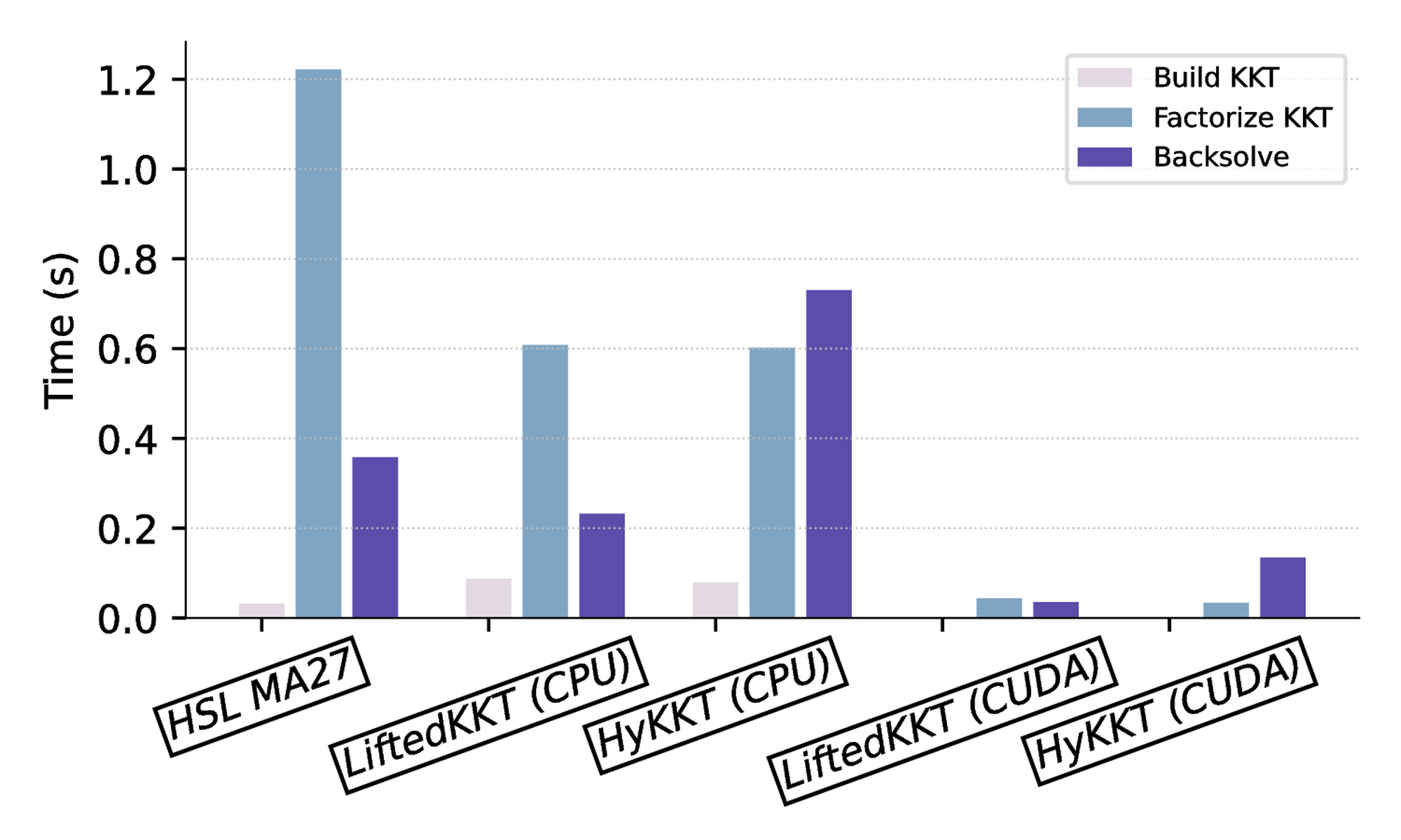
We decompose the time spent in a single IPM iteration for LiftedKKT and HyKKT. As a reference running on the CPU, we show the time spent in the solver HSL MA27. We observe that HSL MA57 is slower than HSL MA27, as the OPF instances are super-sparse. Hence, the block elimination algorithm implemented in HSL MA57 is not beneficial there Personal communication with Iain Duff..

When solving the KKT system, the time can be decomposed into: (1) assembling the KKT system, (2) factorizing the KKT system, and (3) computing the descent direction with triangular solves. As depicted in Figure 2, we observe that constructing the KKT system represents only a fraction of the computation time, compared to the factorization and the triangular solves. Using cuDSS-$ \mathrm{LDL^T}$ , we observe speedups of 30x and 15x in the factorization compared to MA27 and CHOLMOD running on the CPU. Once the KKT system is factorized, computing the descent direction with LiftedKKT is faster than with HyKKT (0.04s compared to 0.13s) as HyKKT has to run a Cg algorithm to solve the Schur complement system (14), leading to additional backsolves in the linear solver.

	build (s)	factorize (s)	backsolve (s)	accuracy
HSL MA27	$ 3.15\times 10^{-2}$	$ 1.22 \times 10^{-0} $	$ 3.58\times 10^{-1}$	$ 5.52\times 10^{-7}$
LiftedKKT (CPU)	$ 8.71\times 10^{-2}$	$ 6.08\times 10^{-1}$	$ 2.32\times 10^{-1}$	$ 3.73\times 10^{-9}$
HyKKT (CPU)	$ 7.97\times 10^{-2}$	$ 6.02\times 10^{-1}$	$ 7.30\times 10^{-1}$	$ 3.38\times 10^{-3}$
LiftedKKT (CUDA)	$ 2.09\times 10^{-3}$	$ 4.37\times 10^{-2}$	$ 3.53\times 10^{-2}$	$ 4.86\times 10^{-9}$
HyKKT (CUDA)	$ 1.86\times 10^{-3}$	$ 3.38\times 10^{-2}$	$ 1.35\times 10^{-1}$	$ 3.91\times 10^{-3}$

Breakdown of the time spent in one IPM iteration
for different linear solvers, when solving <span class="monospace"> 78484epigrids</span> (A30 GPU) — Figure 2. Breakdown of the time spent in one IPM iteration for different linear solvers, when solving 78484epigrids (A30 GPU)

5.3 Benchmark on OPF instances

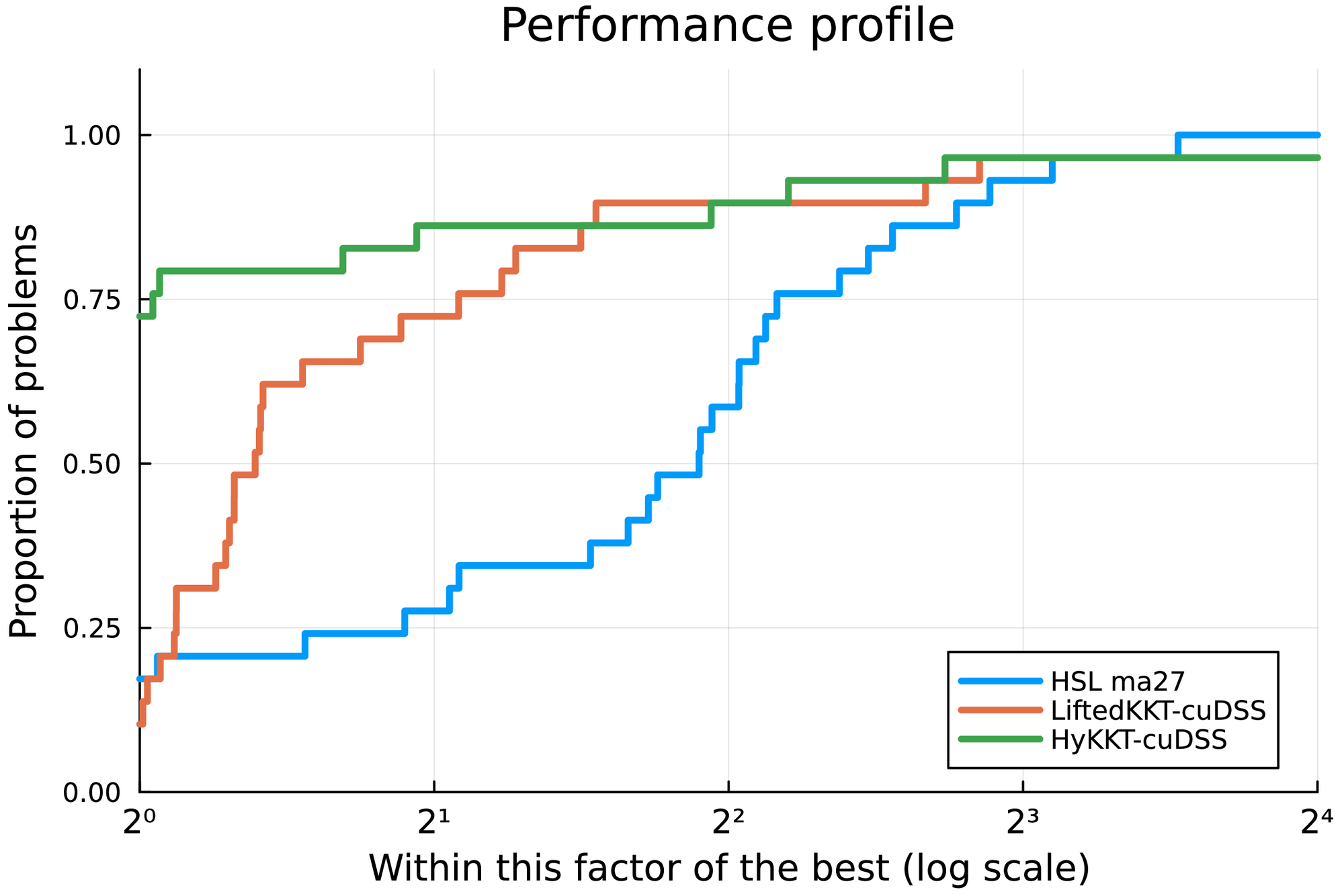
We run a benchmark on difficult OPF instances taken from the PGLIB benchmark [42]. We compare LiftedKKT and HyKKT with HSL MA27. The results are displayed in Table 3, for an IPM tolerance set to $ 10^{-6}$ . Regarding HyKKT, we set $ \gamma = 10^7$ following the analysis in §5.2.2. The table displays the time spent in the initialization, the time spent in the linear solver and the total solving time. We complement the table with a Dolan & Moré performance profile [43] displayed in Figure 3. Overall, the performance of HSL MA27 on the CPU is consistent with what was reported in [42].

On the GPU, LiftedKKT+cuDSS is faster than HyKKT+cuDSS on small and medium instances: indeed, the algorithm does not have to run a Cg algorithm at each IPM iteration, limiting the number of triangular solves performed at each iteration. Both LiftedKKT+cuDSS and HyKKT+cuDSS are significantly faster than HSL MA27. HyKKT+cuDSS is slower when solving 8387_pegase, as on this particular instance the parameter $ \gamma$ is not set high enough to reduce the total number of Cg iterations, leading to a 4x slowdown compared to LiftedKKT+cuDSS. Nevertheless, the performance of HyKKT+cuDSS is better on the largest instances, with almost an 8x speed-up compared to the reference HSL MA27.

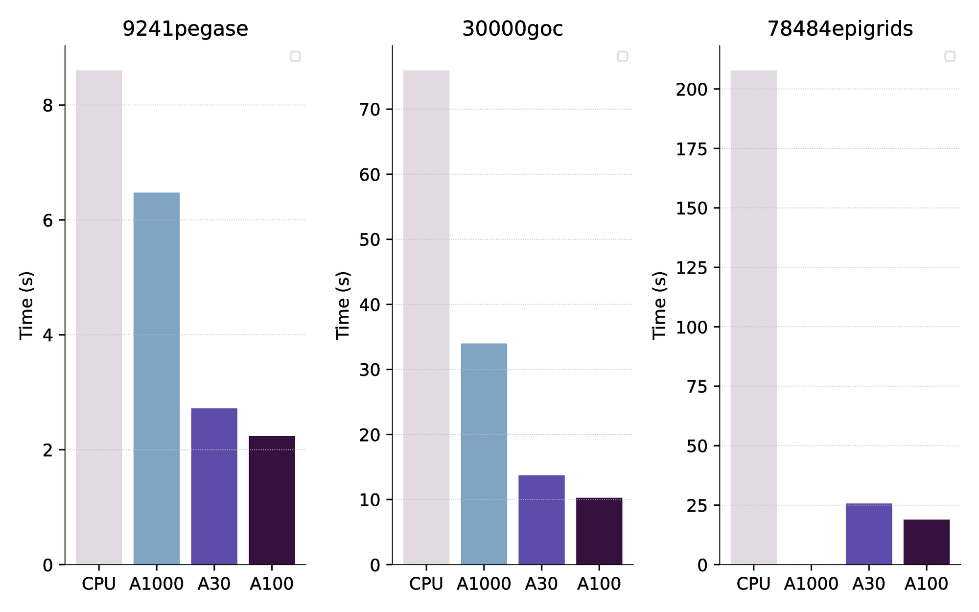
The benchmark presented in Table 3 has been generated using a NVIDIA A100 GPUs (current selling price: $10k). We have also compared the performance with cheaper GPUs: a NVIDIA A1000 (a laptop-based GPU, 4GB memory) and a NVIDIA A30 (24GB memory, price: $5k). As a comparison, the selling price of the AMD EPYC 7443 processor we used for the benchmark on the CPU is $1.2k. The results are displayed in Figure 4. We observe that the performance of the A30 and the A100 are relatively similar. The cheaper A1000 GPU is already faster than HSL MA27 running on the CPU, but is not able to solve the largest instance as it is running out of memory.

Table 3 OPF benchmark, solved with a tolerance tol=1e-6. (A100 GPU)
	HSL MA27				LiftedKKT+cuDSS				HyKKT+cuDSS
Case	it	init	lin	total	it	init	lin	total	it	init	lin	total
89_pegase	32	0.00	0.02	0.03	29	0.03	0.12	0.24	32	0.03	0.07	0.22
179_goc	45	0.00	0.03	0.05	39	0.03	0.19	0.35	45	0.03	0.07	0.25
500_goc	39	0.01	0.10	0.14	39	0.05	0.09	0.26	39	0.05	0.07	0.27
793_goc	35	0.01	0.12	0.18	57	0.06	0.27	0.52	35	0.05	0.10	0.30
1354_pegase	49	0.02	0.35	0.52	96	0.12	0.69	1.22	49	0.12	0.17	0.50
2000_goc	42	0.03	0.66	0.93	46	0.15	0.30	0.66	42	0.16	0.14	0.50
2312_goc	43	0.02	0.59	0.82	45	0.14	0.32	0.68	43	0.14	0.21	0.56
2742_goc	125	0.04	3.76	7.31	157	0.20	1.93	15.49	-	-	-	-
2869_pegase	55	0.04	1.09	1.52	57	0.20	0.30	0.80	55	0.21	0.26	0.73
3022_goc	55	0.03	0.98	1.39	48	0.18	0.23	0.66	55	0.18	0.23	0.68
3970_goc	48	0.05	1.95	2.53	47	0.26	0.37	0.87	48	0.27	0.24	0.80
4020_goc	59	0.06	3.90	4.60	123	0.28	1.75	3.15	59	0.29	0.41	1.08
4601_goc	71	0.09	3.09	4.16	67	0.27	0.51	1.17	71	0.28	0.39	1.12
4619_goc	49	0.07	3.21	3.91	49	0.34	0.59	1.25	49	0.33	0.31	0.95
4837_goc	59	0.08	2.49	3.33	59	0.29	0.58	1.31	59	0.29	0.35	0.98
4917_goc	63	0.07	1.97	2.72	55	0.26	0.55	1.18	63	0.26	0.34	0.94
5658_epigrids	51	0.31	2.80	3.86	58	0.35	0.66	1.51	51	0.35	0.35	1.03
7336_epigrids	50	0.13	3.60	4.91	56	0.45	0.95	1.89	50	0.43	0.35	1.13
8387_pegase	74	0.14	5.31	7.62	82	0.59	0.79	2.30	75	0.58	7.66	8.84
9241_pegase	74	0.15	6.11	8.60	101	0.63	0.88	2.76	71	0.63	0.99	2.24
9591_goc	67	0.20	11.14	13.37	98	0.63	2.67	4.58	67	0.62	0.74	1.96
10000_goc	82	0.15	6.00	8.16	64	0.49	0.81	1.83	82	0.49	0.75	1.82
10192_epigrids	54	0.41	7.79	10.08	57	0.67	1.14	2.40	54	0.67	0.66	1.81
10480_goc	71	0.24	12.04	14.74	67	0.75	0.99	2.72	71	0.74	1.09	2.50
13659_pegase	63	0.45	7.21	10.14	75	0.83	1.05	2.96	62	0.84	0.93	2.47
19402_goc	69	0.63	31.71	36.92	73	1.42	2.28	5.38	69	1.44	1.93	4.31
20758_epigrids	51	0.63	14.27	18.21	53	1.34	1.05	3.57	51	1.35	1.55	3.51
30000_goc	183	0.65	63.02	75.95	-	-	-	-	225	1.22	5.59	10.27
78484_epigrids	102	2.57	179.29	207.79	101	5.94	5.62	18.03	104	6.29	9.01	18.90

Figure 3. Performance profile for the PGLIB OPF benchmark, solved with a tolerance tol=1e-6.

Comparing the performance obtained with various GPUs
on three different OPF instances. — Figure 4. Comparing the performance obtained with various GPUs on three different OPF instances.

5.4 Benchmark on COPS instances

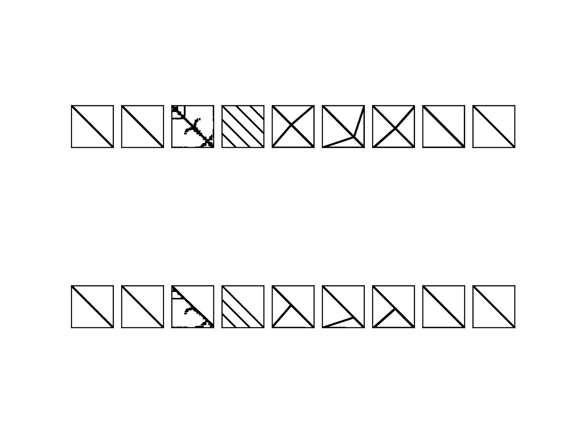
We have observed in the previous section that both LiftedKKT and HyKKT outperforms HSL MA27 when running on the GPU. However, the OPF instances are specific nonlinear instances. For that reason, we complement our analysis by looking at the performance of LiftedKKT and HyKKT on large-scale COPS instances [21]. We look at the performance we get on the COPS instances used in the Mittelmann benchmark [44]. To illustrate the heterogeneity of the COPS instances, we display in Figure 5 the sparsity pattern of the condensed matrices $ K_\gamma$ (13) for one OPF instance and for multiple COPS instances. We observe that some instances ( bearing) have a sparsity pattern similar to the OPF instance on the left, whereas some are fully dense ( elec). On the opposite, the optimal control instances ( marine, steering) are highly sparse and can be reordered efficiently using AMD ordering [37].

The results of the COPS benchmark are displayed in Table 4. HSL MA57 gives better results than HSL MA27 for the COPS benchmark, and for that reason we have decided to replace HSL MA27 by HSL MA57. As expected, the results are different than on the OPF benchmark. We observe that LiftedKKT+cuDSS and HyKKT+cuDSS outperform HSL MA57 on the dense instance elec (20x speed-up) and bearing — an instance whose sparsity pattern is similar to the OPF. In the other instances, LiftedKKT+cuDSS and HyKKT+cuDSS on par with HSL MA57 and sometimes even slightly slower ( rocket and pinene).

Sparsity patterns for one OPF instance and for various
COPS problems. The first row displays the sparsity pattern
of K_) , after AMD reordering. The second row displays
the sparsity pattern of K_) after Metis reordering. — Figure 5. Sparsity patterns for one OPF instance and for various COPS problems. The first row displays the sparsity pattern of $ K_\gamma$ , after AMD reordering. The second row displays the sparsity pattern of $ K_\gamma$ after Metis reordering.

Table 4 COPS benchmark , solved with a tolerance tol=1e-6
			HSL MA57				LiftedKKT+cuDSS				HyKKT+cuDSS
	$ n$	$ m$	it	init	lin	total	it	init	lin	total	it	init	lin	total
bearing_400	162k	2k	17	0.14	3.42	4.10	14	0.85	0.07	1.13	14	0.78	0.76	1.74
camshape_6400	6k	19k	38	0.02	0.18	0.29	35	0.05	0.03	0.19	38	0.05	0.04	0.23
elec_400	1k	0.4k	185	0.54	24.64	33.02	273	0.46	0.97	20.01	128	0.48	0.75	4.16
gasoil_3200	83k	83k	37	0.36	4.81	5.81	21	0.54	0.24	1.40	20	0.59	0.21	1.35
marine_1600	51k	51k	13	0.05	0.41	0.50	33	0.38	0.58	1.29	13	0.37	0.12	0.62
pinene_3200	160k	160k	12	0.11	1.32	1.60	21	0.87	0.16	1.52	11	0.90	0.84	2.02
robot_1600	14k	10k	34	0.04	0.33	0.45	35	0.20	0.07	0.76	34	0.21	0.08	0.80
rocket_12800	51k	38k	23	0.12	1.73	2.16	37	0.74	0.06	2.49	24	0.25	1.70	3.12
steering_12800	64k	51k	19	0.25	1.49	1.93	18	0.44	0.06	1.64	18	0.46	0.07	1.83
bearing_800	643k	3k	13	0.94	14.59	16.86	14	3.31	0.18	4.10	12	3.32	1.98	5.86
camshape_12800	13k	38k	34	0.02	0.34	0.54	33	0.05	0.02	0.16	34	0.06	0.03	0.19
elec_800	2k	0.8k	354	2.36	337.41	409.57	298	2.11	2.58	24.38	184	1.81	2.40	16.33
gasoil_12800	333k	333k	20	1.78	11.15	13.65	18	2.11	0.98	5.50	22	2.99	1.21	6.47
marine_12800	410k	410k	11	0.36	3.51	4.46	146	2.80	25.04	39.24	11	2.89	0.63	4.03
pinene_12800	640k	640k	10	0.48	7.15	8.45	21	4.50	0.99	7.44	11	4.65	3.54	9.25
robot_12800	115k	77k	35	0.54	4.63	5.91	33	1.13	0.30	4.29	35	1.15	0.27	4.58
rocket_51200	205k	154k	31	1.21	6.24	9.51	37	0.83	0.17	8.49	30	0.87	2.67	10.11
steering_51200	256k	205k	27	1.40	9.74	13.00	15	1.82	0.19	5.41	28	1.88	0.56	11.31

6 Conclusion

This article moves one step further in the solution of generic nonlinear programs on GPU architectures. We have compared two approaches to solve the KKT systems arising at each interior-point iteration, both based on a condensation procedure. Despite the formation of an ill-conditioned matrix, our theoretical analysis shows that the loss of accuracy is benign in floating-point arithmetic, thanks to the specific properties of the interior-point method. Our numerical results show that both methods are competitive to solve large-scale nonlinear programs. Compared to the state-of-the-art HSL linear solvers, we achieve a 10x speed-up on large-scale OPF instances and quasi-dense instances (elec). While the results are more varied across the instances of the COPS benchmark, our performance consistently remains competitive with HSL.

Looking ahead, our future plans involve enhancing the robustness of the two condensed KKT methods, particularly focusing on stabilizing convergence for small tolerances (below $ 10^{-8}$ ). It is worth noting that the sparse Cholesky solver can be further customized to meet the specific requirements of the interior-point method [45]. Enhancing the two methods on the GPU would enable the resolution of large-scale problems that are currently intractable on classical CPU architectures such as multiperiod and security-constrained OPF problems.

7 Acknowledgements

This research used resources of the Argonne Leadership Computing Facility, a U.S. Department of Energy (DOE) Office of Science user facility at Argonne National Laboratory and is based on research supported by the U.S. DOE Office of Science-Advanced Scientific Computing Research Program, under Contract No. DE-AC02-06CH11357.

References

[1] Markidis, S., Der Chien, S.W., Laure, E., Peng, I.B., Vetter, J.S.: Nvidia tensor core programmability, performance & precision. In: 2018 IEEE international parallel and distributed processing symposium workshops (IPDPSW), pp. 522–531. IEEE (2018)

[2] Amos, B., Kolter, J.Z.: Optnet: Differentiable optimization as a layer in neural networks. In: International Conference on Machine Learning, pp. 136–145. PMLR (2017)

[3] Pineda, L., Fan, T., Monge, M., Venkataraman, S., Sodhi, P., Chen, R.T., Ortiz, J., DeTone, D., Wang, A., Anderson, S., et al.: Theseus: A library for differentiable nonlinear optimization. Advances in Neural Information Processing Systems 35, 3801–3818 (2022)

[4] Bradbury, J., Frostig, R., Hawkins, P., Johnson, M.J., Leary, C., Maclaurin, D., Necula, G., Paszke, A., VanderPlas, J., Wanderman-Milne, S., Zhang, Q.: JAX: composable transformations of Python+NumPy programs (2018). http://github.com/google/jax

[5] Moses, W.S., Churavy, V., Paehler, L., Hückelheim, J., Narayanan, S.H.K., Schanen, M., Doerfert, J.: Reverse-mode automatic differentiation and optimization of GPU kernels via Enzyme. In: Proceedings of the International Conference for High Performance Computing, Networking, Storage and Analysis, SC '21. Association for Computing Machinery, New York, NY, USA (2021). 10.1145/3458817.3476165. https://doi.org/10.1145/3458817.3476165

[6] Shin, S., Pacaud, F., Anitescu, M.: Accelerating optimal power flow with GPUs: SIMD abstraction of nonlinear programs and condensed-space interior-point methods. arXiv preprint arXiv:2307.16830 (2023)

[7] Lu, H., Yang, J.: cuPDLP.jl: A GPU implementation of restarted primal-dual hybrid gradient for linear programming in julia. arXiv preprint arXiv:2311.12180 (2023)

[8] Lu, H., Yang, J., Hu, H., Huangfu, Q., Liu, J., Liu, T., Ye, Y., Zhang, C., Ge, D.: cuPDLP-C: A strengthened implementation of cuPDLP for linear programming by C language. arXiv preprint arXiv:2312.14832 (2023)

[9] Kim, Y., Pacaud, F., Kim, K., Anitescu, M.: Leveraging GPU batching for scalable nonlinear programming through massive Lagrangian decomposition (2021). 10.48550/arXiv.2106.14995

[10] Świrydowicz, K., Darve, E., Jones, W., Maack, J., Regev, S., Saunders, M.A., Thomas, S.J., Peleš, S.: Linear solvers for power grid optimization problems: a review of GPU-accelerated linear solvers. Parallel Computing p. 102870 (2021)

[11] Tasseff, B., Coffrin, C., Wächter, A., Laird, C.: Exploring benefits of linear solver parallelism on modern nonlinear optimization applications. arXiv preprint arXiv:1909.08104 (2019)

[12] Curtis, F.E., Huber, J., Schenk, O., Wächter, A.: A note on the implementation of an interior-point algorithm for nonlinear optimization with inexact step computations. Mathematical Programming 136(1), 209–227 (2012). 10.1007/s10107-012-0557-4

[13] Rodriguez, J.S., Laird, C.D., Zavala, V.M.: Scalable preconditioning of block-structured linear algebra systems using ADMM. Computers & Chemical Engineering 133, 106478 (2020). 10.1016/j.compchemeng.2019.06.003

[14] Ghannad, A., Orban, D., Saunders, M.A.: Linear systems arising in interior methods for convex optimization: a symmetric formulation with bounded condition number. Optimization Methods and Software 37(4), 1344–1369 (2022)

[15] Cao, Y., Seth, A., Laird, C.D.: An augmented lagrangian interior-point approach for large-scale NLP problems on graphics processing units. Computers & Chemical Engineering 85, 76–83 (2016)

[16] Regev, S., Chiang, N.Y., Darve, E., Petra, C.G., Saunders, M.A., Świrydowicz, K., Peleš, S.: HyKKT: a hybrid direct-iterative method for solving KKT linear systems. Optimization Methods and Software 38(2), 332–355 (2023)

[17] Golub, G.H., Greif, C.: On solving block-structured indefinite linear systems. SIAM Journal on Scientific Computing 24(6), 2076–2092 (2003)

[18] Pacaud, F., Shin, S., Schanen, M., Maldonado, D.A., Anitescu, M.: Accelerating condensed interior-point methods on SIMD/GPU architectures. Journal of Optimization Theory and Applications pp. 1–20 (2023)

[19] Wright, M.H.: Ill-conditioning and computational error in interior methods for nonlinear programming. SIAM Journal on Optimization 9(1), 84–111 (1998)

[20] Montoison, A.: CUDSS.jl: Julia interface for NVIDIA cuDSS. https://github.com/exanauts/CUDSS.jl

[21] Dolan, E.D., Moré, J.J., Munson, T.S.: Benchmarking optimization software with COPS 3.0. Tech. rep., Argonne National Lab., Argonne, IL (US) (2004)

[22] Nocedal, J., Wright, S.J.: Numerical optimization, 2nd edn. Springer series in operations research. Springer, New York (2006)

[23] Benzi, M., Golub, G.H., Liesen, J.: Numerical solution of saddle point problems. Acta numerica 14, 1–137 (2005)

[24] Wächter, A., Biegler, L.T.: On the implementation of an interior-point filter line-search algorithm for large-scale nonlinear programming. Mathematical Programming 106(1), 25–57 (2006)

[25] Duff, I.S., Reid, J.K.: The multifrontal solution of indefinite sparse symmetric linear. ACM Transactions on Mathematical Software (TOMS) 9(3), 302–325 (1983)

[26] Gondzio, J.: Interior point methods 25 years later. European Journal of Operational Research 218(3), 587–601 (2012). 10.1016/j.ejor.2011.09.017

[27] Waltz, R.A., Morales, J.L., Nocedal, J., Orban, D.: An interior algorithm for nonlinear optimization that combines line search and trust region steps. Mathematical Programming 107(3), 391–408 (2006)

[28] Duff, I.S.: MA57—a code for the solution of sparse symmetric definite and indefinite systems. ACM Transactions on Mathematical Software (TOMS) 30(2), 118–144 (2004)

[29] Debreu, G.: Definite and semidefinite quadratic forms. Econometrica: Journal of the Econometric Society pp. 295–300 (1952)

[30] Hestenes, M.R., Stiefel, E.: Methods of conjugate gradients for solving linear systems. Journal of Research of the National Bureau of Standards 49(6), 409–436 (1952). 10.6028/jres.049.044

[31] Montoison, A., Orban, D., Saunders, M.A.: MinAres: An iterative solver for symmetric linear systems. Les Cahiers du GERAD G-2023-40, Groupe d’études et de recherche en analyse des décisions (2023)

[32] Wright, S.J.: Effects of finite-precision arithmetic on interior-point methods for nonlinear programming. SIAM Journal on Optimization 12(1), 36–78 (2001)

[33] Stewart, G.W., Sun, J.g.: Matrix perturbation theory. (No Title) (1990)

[34] Bezanson, J., Edelman, A., Karpinski, S., Shah, V.B.: Julia: A fresh approach to numerical computing. SIAM Review 59(1), 65–98 (2017). 10.1137/141000671

[35] Shin, S., Coffrin, C., Sundar, K., Zavala, V.M.: Graph-based modeling and decomposition of energy infrastructures. IFAC-PapersOnLine 54(3), 693–698 (2021)

[36] Bischof, C., Griewank, A., Juedes, D.: Exploiting parallelism in automatic differentiation. In: Proceedings of the 5th international conference on Supercomputing, pp. 146–153 (1991)

[37] Amestoy, P.R., Davis, T.A., Duff, I.S.: Algorithm 837: AMD, an approximate minimum degree ordering algorithm. ACM Transactions on Mathematical Software (TOMS) 30(3), 381–388 (2004)

[38] Chen, Y., Davis, T.A., Hager, W.W., Rajamanickam, S.: Algorithm 887: CHOLMOD, supernodal sparse cholesky factorization and update/downdate. ACM Transactions on Mathematical Software (TOMS) 35(3), 1–14 (2008)

[39] Fowkes, J., Lister, A., Montoison, A., Orban, D.: LibHSL: the ultimate collection for large-scale scientific computation. Les Cahiers du GERAD G-2024-06, Groupe d’études et de recherche en analyse des décisions (2024)

[40] Montoison, A., Orban, D., contributors: HSL.jl: A Julia interface to the HSL mathematical software library. https://github.com/JuliaSmoothOptimizers/HSL.jl (2021). 10.5281/zenodo.2658672

[41] Montoison, A., Orban, D.: Krylov. jl: A julia basket of hand-picked Krylov methods. Journal of Open Source Software 8(89), 5187 (2023)

[42] Babaeinejadsarookolaee, S., Birchfield, A., Christie, R.D., Coffrin, C., DeMarco, C., Diao, R., Ferris, M., Fliscounakis, S., Greene, S., Huang, R., et al.: The power grid library for benchmarking AC optimal power flow algorithms. arXiv preprint arXiv:1908.02788 (2019)

[43] Dolan, E.D., Moré, J.J.: Benchmarking optimization software with performance profiles. Mathematical programming 91, 201–213 (2002)

[44] Mittelmann, H.D.: Benchmark for optimization software (2002). http://plato. asu. edu/bench. html

[45] Wright, S.J.: Modified cholesky factorizations in interior-point algorithms for linear programming. SIAM Journal on Optimization 9(4), 1159–1191 (1999)

linear solver	analysis (s)	factorization (s)	backsolve (s)	abs. accuracy
CHOLMOD	1.18	\( 8.57 \times 10^{-1}\)	\( 1.27 \times 10^{-1}\)	\( 3.60\times 10^{-13}\)
cuDSS-Cholesky	4.52	\( 3.75 \times 10^{-2}\)	\( 1.32 \times 10^{-2}\)	\( 2.64\times 10^{-13}\)
cuDSS-\( \mathrm{LU}\)	4.50	\( 3.72 \times 10^{-2}\)	\( 1.49 \times 10^{-2}\)	\( 2.58\times 10^{-13}\)
cuDSS-\( \mathrm{LDL^T}\)	4.50	\( 4.07 \times 10^{-2}\)	\( 1.55 \times 10^{-2}\)	\( 7.62\times 10^{-11}\)

	build (s)	factorize (s)	backsolve (s)	accuracy
HSL MA27	\( 3.15\times 10^{-2}\)	\( 1.22 \times 10^{-0} \)	\( 3.58\times 10^{-1}\)	\( 5.52\times 10^{-7}\)
LiftedKKT (CPU)	\( 8.71\times 10^{-2}\)	\( 6.08\times 10^{-1}\)	\( 2.32\times 10^{-1}\)	\( 3.73\times 10^{-9}\)
HyKKT (CPU)	\( 7.97\times 10^{-2}\)	\( 6.02\times 10^{-1}\)	\( 7.30\times 10^{-1}\)	\( 3.38\times 10^{-3}\)
LiftedKKT (CUDA)	\( 2.09\times 10^{-3}\)	\( 4.37\times 10^{-2}\)	\( 3.53\times 10^{-2}\)	\( 4.86\times 10^{-9}\)
HyKKT (CUDA)	\( 1.86\times 10^{-3}\)	\( 3.38\times 10^{-2}\)	\( 1.35\times 10^{-1}\)	\( 3.91\times 10^{-3}\)

	CHOLMOD-\( \mathrm{LDL^T}\) (CPU)					cuDSS-\( \mathrm{LDL^T}\) (CUDA)
\( \gamma\)	# it	cond. (s)	Cg (s)	linsol (s)	IPM (s)	# it	cond. (s)	Cg (s)	linsol (s)	IPM (s)
\( 10^4\)	96	8.15	463.86	536.83	575.06	96	0.17	113.27	114.52	124.00
\( 10^5\)	96	8.33	163.35	235.61	273.36	96	0.17	53.37	54.62	64.39
\( 10^6\)	96	8.22	68.69	139.86	177.24	96	0.17	14.53	15.78	25.39
\( 10^7\)	96	8.24	35.12	107.17	144.78	96	0.17	7.95	9.20	18.41
\( 10^8\)	96	7.89	21.68	93.85	131.33	96	0.17	5.36	6.62	15.90

	CHOLMOD-\( \mathrm{LDL^T}\) (CPU)		cuDSS-\( \mathrm{LDL^T}\) (CUDA)
\( \varepsilon_{tol}\)	#it	time (s)	#it	time (s)	accuracy
\( 10^{-4}\)	115	268.2	114	19.9	\( 1.2 \times 10^{-2}\)
\( 10^{-5}\)	210	777.8	113	30.4	\( 1.2 \times 10^{-3}\)
\( 10^{-6}\)	102	337.5	109	25.0	\( 1.2 \times 10^{-4}\)
\( 10^{-7}\)	108	352.9	104	20.1	\( 1.2 \times 10^{-5}\)
\( 10^{-8}\)	-	-	105	20.3	\( 1.2 \times 10^{-6}\)

Dynamic display of documents.

Collapse and expand sections

Cross-references and related material

Discussions

Table of contents

Abstract

1 Introduction

1.1 Solving optimization problems on GPU: current state-of-the-art

1.1.1 GPU for mathematical programming.

1.1.2 GPU for batched optimization solvers.

1.1.3 GPU for nonlinear programming.

1.2 Contributions

1.3 Notations

2 Primal-dual interior-point method

2.1 Problem formulation and KKT conditions

2.2 Solving the KKT conditions with the interior-point method

2.2.1 Augmented KKT system.

2.2.2 Condensed KKT system.

2.2.3 Iterative refinement.

2.3 Discussion

3 Solving KKT systems on the GPU

3.1 Golub & Greif strategy: HyKKT

3.2 Equality relaxation strategy: LiftedKKT

3.3 Discussion

4 Conditioning of the condensed KKT system

4.1 Centrality conditions

4.2 Structured ill-conditioning

4.2.1 Invariant subspaces in \( K_\gamma\)

4.2.2 Numerical accuracy of the condensed matrix \( K_\gamma\)

4.2.3 Numerical solution of the condensed system

4.2.3.1 Impact of right-hand-side perturbation.

4.2.3.2 Impact of matrix perturbation.

4.3 Solution of the condensed KKT system

4.3.1 Solution with HyKKT

4.3.1.1 Initial right-hand-side.

4.3.1.2 Schur-complement operator.

4.3.2 Solution with Lifted KKT system

4.3.3 Summary

5 Numerical results

5.1 Implementation

5.1.1 IPM solver.

5.1.2 Evaluation of the nonlinear models.

5.1.3 Linear solvers.

5.2 Performance analysis on a large-scale instance

5.2.1 Individual performance of the linear solvers

5.2.2 Tuning the Golub & Greif strategy

5.2.3 Tuning the equality relaxation strategy

5.2.4 Breakdown of the time spent in one IPM iteration

5.3 Benchmark on OPF instances

5.4 Benchmark on COPS instances

6 Conclusion

7 Acknowledgements

References

Discussion: create topic login to participate.