In this article, we address the problem of federated learning in the presence of stragglers. For this problem, a coded federated learning framework has been proposed, where the central server aggregates gradients received from the non-stragglers and gradient computed from a privacy-preservation global coded dataset to mitigate the negative impact of the stragglers. However, when aggregating these gradients, fixed weights are consistently applied across iterations, neglecting the generation process of the global coded dataset and the dynamic nature of the trained model over iterations. This oversight may result in diminished learning performance. To overcome this drawback, we propose a new method named adaptive coded federated learning (ACFL). In ACFL, before the training, each device uploads a coded local dataset with additive noise to the central server to generate a global coded dataset under privacy preservation requirements. During each iteration of the training, the central server aggregates the gradients received from the non-stragglers and the gradient computed from the global coded dataset, where an adaptive policy for varying the aggregation weights is designed. Under this policy, we optimize the performance in terms of privacy and learning, where the learning performance is analyzed through convergence analysis and the privacy performance is characterized via mutual information differential privacy. Finally, we perform simulations to demonstrate the superiority of ACFL compared with the non-adaptive methods.

In intelligent systems, edge devices are generating an increasing amount of data, which can be utilized to train machine learning models for various tasks across a wide range of applications, such as smart cities [1], autonomous driving [2], and intelligent healthcare [3]. Traditionally, these data are uploaded to a central server for centralized machine learning. However, uploading datasets directly to the central server without privacy-preservation measures raises severe privacy concerns for the edge devices [4]. As an alternative to centralized machine learning, federated learning (FL) has emerged as a highly effective tool [5, 6, 7]. Under the FL framework, during each iteration of the training process, local devices compute gradients with their local datasets and send these gradients to a central server. The central server then aggregates the received gradients to update the global model [8]. In this manner, the edge devices only share locally computed gradients with the central server, significantly enhancing the privacy of raw datasets.

In FL, the training process may be hindered by devices known as stragglers, which are significantly slower than others or completely unresponsive due to various incidents [9, 10]. Additionally, in FL, the local datasets on different devices can be highly heterogeneous, meaning they are not independent and identically distributed (non-i.i.d.) across devices [11, 12]. In this case, the presence of stragglers can bias the trained global model due to the absence of the contributions of some devices in each iteration. In other words, stragglers can negatively impact the learning performance of FL, potentially leading to poor convergence. In traditional distributed learning scenarios, the challenges posed by stragglers can be addressed through well-known gradient coding (GC) strategies [13, 14, 15, 16, 17, 18, 19]. The core concept of GC is replicating the training data samples and distributing them redundantly across the devices prior to training. During each training iteration, non-straggler devices encode the locally computed gradients and transmit the encoded vectors to the central server. Upon receiving these vectors, the central server is able to reconstruct the global gradient, effectively mitigating the impact of stragglers. However, in FL scenarios, privacy concerns make it impractical to adopt GC techniques and to allocate training data to devices redundantly in a carefully planned manner, as is done in traditional distributed learning scenarios. This is because devices are reluctant to share their local datasets directly with others to create data redundancy considering that their local datasets may contain sensitive or private information [20].

For FL problems, to evade the negative impact of stragglers, a new paradigm named coded federated learning (CFL) has been investigated [21, 22, 23, 24]. In CFL, each device uploads a coded version of its dataset to the central server to form a global coded dataset before training begins. During the training process, the central server aggregates gradients received from the non-stragglers and gradient computed from the global coded dataset to mitigate the negative impact of the stragglers. Compared with sharing raw datasets as in GC, by carefully designing the way of encoding local datasets in CFL, privacy concerns can be largely reduced, and one can even achieve perfect privacy. However, it is intuitive that encoding the local datasets induces information loss and this may negatively impacts the learning performance. Based on that, the key issue in CFL is how to generate the global coded dataset before training, as well as how to aggregate the gradients at the central server during the training process, in order to achieve better performance in terms of learning and privacy.

There has been some recent progress under the framework of CFL. To be more specific, CFL was firstly investigated in [21] for linear regression problems under the FL setting, where local coded datasets are constructed at the devices by applying random linear projections. In [22], the CFL scheme was combined with distributed kernel embedding to make CFL applicable for nonlinear FL problems. Later, to further enhance the privacy performance of CFL, a differentially private CFL method was proposed by adding noise to the local coded datasets, where the differential privacy guarantee was proved [23]. Very recently, a stochastic coded federated learning (SCFL) method has been proposed [24]. In SCFL, before the training starts, the devices generate and upload privacy-preservation coded datasets to the central server by adding noise to the projected local datasets, which are used by the central server to generate the global coded dataset. In each iteration of the training process, the central server aggregates gradients received from the non-stragglers and gradient computed from the global coded dataset with fixed aggregation weights. Compared with previous methods, the advantages of SCFL lie in ensuring that the global gradient applied by the central server to update the global model is an unbiased estimation of the true gradient, and providing the trade off between the privacy performance and the learning performance analytically. However, in SCFL, when the central server aggregates the gradients, it consistently adopts pre-specified and fixed weights across iterations, which neglects the generation process of the global coded dataset and the dynamic nature of the trained model over iterations. This oversight results in an unnecessary performance loss, preventing SCFL from achieving the optimal performance in terms of privacy and learning.

For FL under requirements of privacy preservation and straggler mitigation, to overcome the drawbacks of existing CFL methods as mentioned above, we propose a new method named adaptive coded federated learning (ACFL). In ACFL, before training, each device uploads a local coded dataset, which is a transformed version of its local dataset with added random noise. Upon receiving local coded datasets from the devices, the central server generates the global coded dataset. Then, during each training iteration, each non-straggler device computes local gradient based on the current global model and its local dataset, subsequently transmitting this gradient to the central server. After receiving local gradients from the non-straggler devices, the central server estimates the global gradient by aggregating the received gradients and the gradient computed from the global coded dataset, applying aggregation weights determined by an adaptive policy. Under this policy, the performance in terms of privacy and learning is optimized, where the learning performance is described by convergence analysis and the privacy performance is measured by mutual information differential privacy (MI-DP). Finally, in order to verify the superiority of the proposed method, simulations results are provided, where we compare the performance of ACFL and the non-adaptive methods.

Our contributions are summarized as follows:

1. We propose a new ACFL method designed for FL problems under requirements of straggler mitigation and privacy preservation. This method develops an adaptive policy for adjusting the aggregation weights at the central server during gradient aggregation, aiming to achieve the optimal performance in terms of privacy and learning.
2. We analytically analyze the trade off between learning and privacy performance of the proposed method.
3. Through simulations, we demonstrate that the proposed method surpasses the non-adaptive methods, which attains better learning performance while maintaining the same level of privacy concerns.

The rest of this paper is structured as follows. In Section 2, we formulate the considered problem. In Section 3, we propose our ACFL method. In Section 4, we analyze the performance of ACFL theoretically and describes the adaptive policy adopted by the proposed method. Simulation results are provided in Section 5 to verify the superiority of the proposed method. Finally, we conclude this paper in Section 6.

In the FL system, there is a central server and \(N\) devices, where each device \(i\) owns a local dataset consisting of \({{\mathbf{X}}^{(i)}} \in \mathbb{R}^{m_i \times d}\) and \({{\mathbf{Y}}^{(i)}} \in \mathbb{R}^{m_i \times o}\), \(\forall i\). Here, \({{\mathbf{X}}^{(i)}}\) contains \(m_i\) data samples of dimension \(d\), and \({{\mathbf{Y}}^{(i)}}\) represents the corresponding labels of dimension \(o\). We also assume that, for each local dataset, the number of data samples \(m_i\) is greater than \(d\) and \({{\mathbf{X}}^{(i)}} \in \mathbb{R}^{m_i \times d}\) is full column rank [25]. Under the coordination of the central server, the aim is to minimize the total training loss \( f\left( \mathbf{W} \right)\) by finding the solution to the following linear regression problem [24]:

where \(\mathbf{W} \in \mathbb{R}^{d \times o}\) is the model parameter matrix, and \(\left\| \cdot \right\|_F\) denotes the Frobenius norm. Here, we focus on linear regression problems under the FL setting for two reasons. First, linear regression is a very important machine learning model that has attracted significant attention recently due to its ability to make scientific and reliable predictions. As a statistical procedure established a long time ago, its properties are well understood, enabling the rapid training of linear regression models in different applications [26, 27, 28, 29]. Second, nonlinear problems can be transformed into linear regression problems through kernel embedding methods, demonstrating the broad applicability of linear regression models, as indicated by [30].

For the problem introduced above under the FL setting, the training process involves multiple iterations. In each iteration, each device computes local gradient based on its local dataset and transmits it to the central server. After aggregating the received gradients, the central server updates the global model and broadcasts the model parameters to all devices. Over the iterations, due to various incidents, some devices may become stragglers, which are temporarily unresponsive, fail to implement computations, and do not send any messages to the central server, unlike the normally functioning devices [13]. It is assumed that the probability of each device being a straggler is \( p\) in each iteration, and the straggler behavior of the devices is independent across iterations and among different devices [19]. It is obvious that the presence of stragglers may degrade the learning performance or even leads to very poor convergence.

To deal with the stragglers in FL, the CFL paradigm has been studied. In CFL, the local dataset \(\left( {\mathbf{X}^{(i)},\mathbf{Y}^{(i)}} \right)\) is encoded into \(\left( {\mathbf{H}_X^{(i)},\mathbf{H}_Y^{(i)}} \right)\) and transmitted to the central server by device \(i\) before training begins, \(\mathbf{H}_X^{(i)} \in \mathbb{R}^{n_X^{(i)} \times d}\), \(\mathbf{H}_Y^{(i)} \in \mathbb{R}^{n_Y^{(i)} \times o}\), \( \forall i\) . The central server utilizes the local coded datasets to generate a global coded dataset, denoted as \(\left( \mathbf{\tilde H}_X, \mathbf{\tilde H}_Y \right)\), instead of retaining all the received coded datasets to save its storage [24]. Subsequently, the training process begins, involving multiple iterations. In each iteration, each non-straggler device computes the gradient based on its local dataset and transmits it to the central server. Upon receiving these messages from the non-stragglers, the central server updates the current model parameter matrix using both the received gradients and the gradient computed from the global coded dataset [24]. At the end of each iteration, the central server broadcasts the updated model parameters to all devices. In CFL, the core issue is to design the method of generating global coded dataset before training and aggregating gradients at the central server during the training process, so that we can achieve a better performance in terms of privacy and learning. A recently proposed method within the CFL framework is known as SCFL [24], which generates local coded datasets by adding noise and random projections. The global dataset is then assembled as the sum of these local coded datasets. Throughout each training iteration, the central server employs a weighted sum with fixed and pre-specified weights across all iterations to aggregate the gradients. However, in SCFL, consistently using fixed and pre-specified weights for aggregating gradients without considering the generation process of the global coded dataset and the dynamic nature of the trained model over iterations results in an unnecessary performance loss.

To overcome the limitations of the existing work, our aim is to attain a better performance in terms of privacy and learning for FL problems under the requirements of privacy preservation and straggler mitigation.

In this section, we propose the ACFL method to address the problem outlined in Section 2. ACFL is implemented in two distinct stages. Initially, in the first stage prior to the commencement of training, each device transmits a coded dataset to the central server, which is derived by transforming its local dataset and adding noise. The central server then uses these local coded datasets to generate a global coded dataset. Subsequently, in the second stage, the training process involves multiple iterations. In each iteration, the central server aggregates gradient computed from the global coded dataset and the received gradients from non-straggler devices, where an adaptive policy to determine the aggregation weights is applied.

3.1 The first stage: before training

3.2 The second stage: training iterations

In this section, we first analyze the performance of the proposed method with arbitrary aggregation weights from two aspects: privacy performance and learning performance. Based on that, to attain the optimal performance in terms of privacy and learning, the adaptive policy of determining the value of \( \alpha_t\) would be specified accordingly. First, let us provide some useful assumptions, which have been widely and reasonably adopted in the literature.

4.1 Privacy performance of ACFL

4.2 Learning performance of ACFL

4.3 The adaptive policy

Based on Section 4.1 and Section 4.2, let us now consider how to adaptively determine the value of \( \alpha_t\) for ACFL to attain a better performance in terms of privacy and learning. According to Theorem 1 and Theorem 2, the problem of determining \( \alpha _t\) in ACFL can be equivalently expressed as the following optimization problem:

\[ \begin{align} {\min }\limits_{{\alpha _t}} u\left( {\sigma _1^2,\sigma _2^2,{\alpha _t}} \right), s.t. 0\leq{\alpha _t}\leq1, \end{align} \]

(37)

which aims to expedite the convergence of the learning process under certain privacy level with fixed variances of additive noise. Based on the optimization problem defined in (37), we detail the adaptive policy for selecting the value of \(\alpha_t\) and analyze the trade off between privacy and learning performance under this policy in Theorem 3 as follows.

Theorem 3

For the proposed ACFL method, by setting

\[ \begin{align} \alpha_t= \frac{{pN{\beta ^2}\frac{1}{{1 - p}}}}{{pN{\beta ^2}\frac{1}{{1 - p}} + Nd\sigma _1^2{C^2} + N\sigma _2^2od}}, \end{align} \]

(38)

the optimal performance in terms of privacy and learning can be attained. In this case, under Assumptions 1-3, if \( \sum\limits_{i = 1}^N {{{\mathbf{X}}^{\left( i \right)}}^T{{\mathbf{X}}^{\left( i \right)}}} \geq \lambda {\mathbf{I}}\) with \( \lambda>0\) , by setting \( {\eta _t} = {1 \left/ {\vphantom {1 {\left( {\lambda t} \right)}}} \right. - {\left( {\lambda t} \right)}}\) , it holds that

\[ \begin{align} \mathbb{E}\left( {\left\| {{{\mathbf{W}}_T} - {{\mathbf{W}}^*}} \right\|_F^2} \right) \leqslant 4\frac{{\tilde u\left( {\sigma _1^2,\sigma _2^2} \right)}}{{{\lambda ^2}T}}, \end{align} \]

(39)

where

\[ \begin{align} & \tilde u\left( {\sigma _1^2,\sigma _2^2} \right) \nonumber \end{align} \]

(40)

\[ \begin{align} =& - \frac{{{{\left( {pN{\beta ^2}\frac{1}{{1 - p}}} \right)}^2}}}{{N{\beta ^2}p\frac{1}{{1 - p}} + Nd\sigma _1^2{C^2} + N\sigma _2^2od}} \\ &+ N{\beta ^2}\frac{1}{{1 - p}} + N{\beta ^2}\left( {N - 1} \right), \\\end{align} \]

With the learning performance provided as (39) and the privacy performance described in Theorem 1, the performance in terms of privacy and learning attained by the proposed method is characterized.

Proof

Problem (37) can be equivalently expressed as the following optimization problem:

\[ \begin{align} {\min }\limits_{{\alpha _t}} \hat u\left( {{\alpha _t}} \right),s.t.0 \leqslant {\alpha _t} \leqslant 1, \end{align} \]

(41)

where

\[ \begin{align} \hat u\left( {{\alpha _t}} \right) \triangleq& \alpha _t^2\left( {N{\beta ^2}p\frac{1}{{1 - p}} + Nd\sigma _1^2{C^2} + N\sigma _2^2od} \right) \nonumber \end{align} \]

(42)

\[ \begin{align} &- \left( {2pN{\beta ^2}\frac{1}{{1 - p}}} \right){\alpha _t}. \\\end{align} \]

(43)

Noting that \( \frac{{pN{\beta ^2}\frac{1}{{1 - p}}}}{{\left( {pN{\beta ^2}\frac{1}{{1 - p}} + Nd\sigma _1^2{C^2} + N\sigma _2^2od} \right)}} < 1\) always holds, which indicates that

\[ \begin{align} & {\arg \min }\lim_{\alpha _t} \hat u\left( {{\alpha _t}} \right) \nonumber \end{align} \]

(44)

\[ \begin{align} &= \frac{{pN{\beta ^2}\frac{1}{{1 - p}}}}{{pN{\beta ^2}\frac{1}{{1 - p}} + Nd\sigma _1^2{C^2} + N\sigma _2^2od}}. \\\end{align} \]

(45)

Substituting (44) into (36) yields (39), which completes the proof.

Remark 4

According to Theorem 3, the learning performance of ACFL improves as the variances of the additive noise decrease, whereas the privacy performance benefits from an increase in these variances. This highlights the intrinsic trade off between privacy and learning performance. Practically, the variances of the additive noise can be meticulously calibrated to achieve a desired trade off, aligning with specific practical requirements.

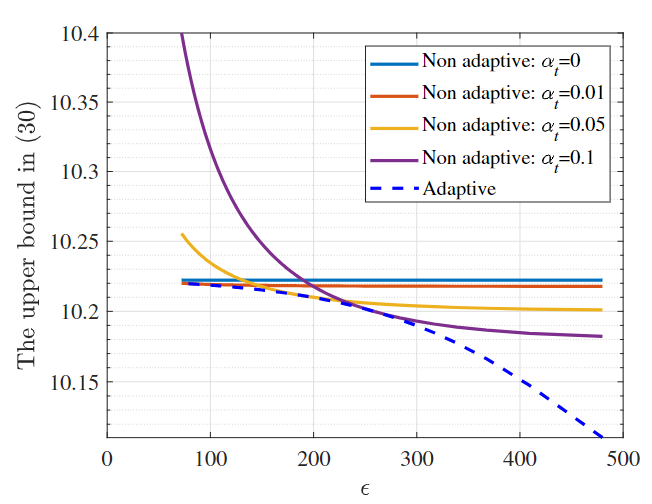
To verify that ACFL with the adaptive policy achieves a better performance in terms of privacy and learning, Fig. 1 illustrates the relationship between the upper bound derived in (35) and \(\epsilon\) specified in (17) with non-adaptive and fixed values of aggregation weights as well as adaptive aggregation weights determined by the designed adaptive policy, where we set \( d=100, \sigma_1^2=\sigma^2_2, o=10, p=0.1, N=5, \beta=10, c=1, T=1000\) and \( \lambda=1\) . Here, a lower value of the upper bound implies superior learning performance, whereas a lower \(\epsilon\) value signifies enhanced privacy performance. The results clearly show that under equivalent privacy levels, the upper bound in (35) reaches its minimum with the adaptive policy. This outcome indicates that ACFL, when implemented with the adaptive policy, attains the optimal performance in terms of privacy and learning.

In Theorem 3, we develop the adaptive policy for setting the aggregation weights in ACFL, which relies on the bounds specified in Assumptions 2 and 3. Notably, obtaining the values of \(C\) and \(\beta\) beforehand can be challenging in certain scenarios. In such cases, a practical implementation of ACFL involves estimating \(C\) and \(\beta\) over the iterations by the central server. Specifically, \(C\) and \(\beta\) are approximated by \(\hat{C}\) and \(\hat{\beta}\), respectively, with their expressions provided as follows:

\[ \begin{align} \hat{C}^2 = \left\| {{{\mathbf{W}}_t}} \right\|_F^2, \hat{\beta}^2 = \frac{{\sum\limits_{i = 1}^N {\left\| {{\mathbf{G}}_t^{\left( i \right)}} \right\|_F^2I_t^{\left( i \right)}} }}{{\sum\limits_{i = 1}^N {I_t^{\left( i \right)}} }}. \end{align} \]

(46)

Based on (46), the aggregation weights can be determined adaptively as

\[ \begin{align} {{\overset{\lower0.5em \( \smash{\scriptscriptstyle\smile}\) }{\alpha } }_t} = \frac{{p{{\hat \beta }^2}}}{{p{{\hat \beta }^2} + d\sigma _1^2{{\hat C}^2}\left( {1 - p} \right) + \sigma _2^2od\left( {1 - p} \right)}}. \end{align} \]

(47)

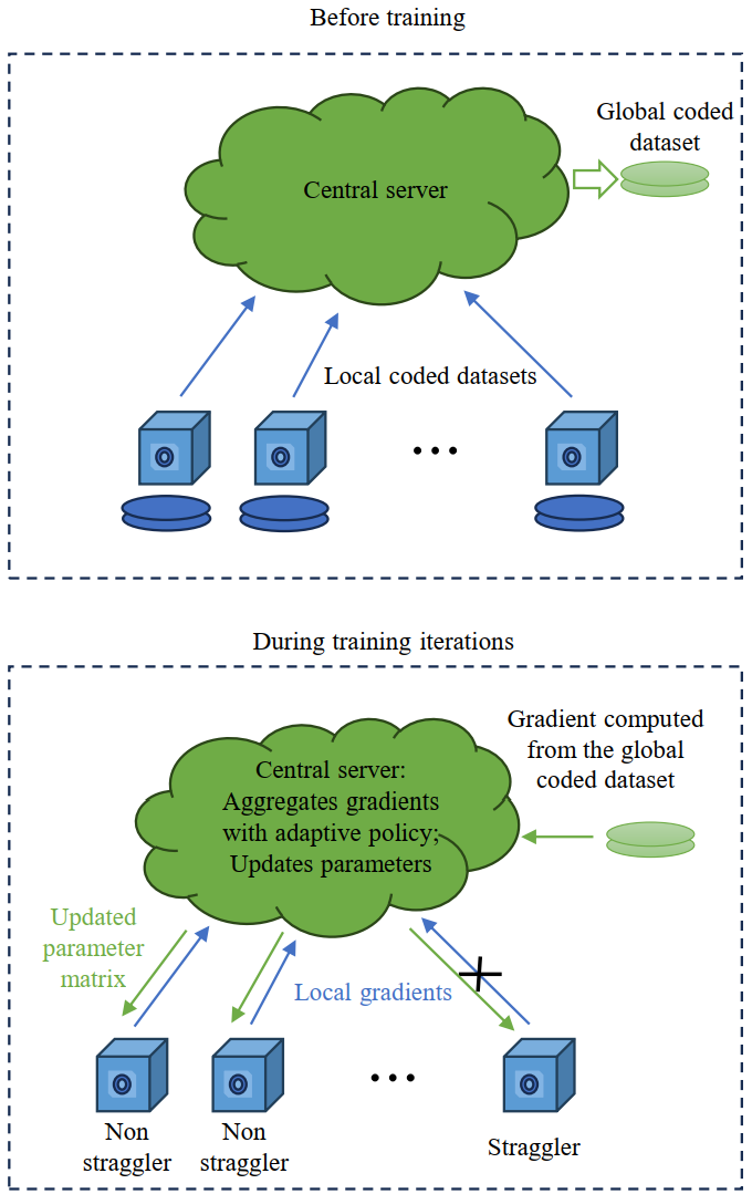
With (47), the implementation of ACFL is presented in Algorithm 1 and shown as Fig. 4.

---

Algorithm 1 ACFL

---

1.Input: Initial parameter matrix \({\mathbf{W}}_0\), learning rates \( \eta_t\)

2.The first stage: Device \( i\) uploads coded dataset \(\left( {\mathbf{H}_X^{(i)},\mathbf{H}_Y^{(i)}} \right)\) to the central server as (2) and (3), \( \forall i\) .

3.The central server generates a global coded dataset \(\left( {{{{\mathbf{\tilde H}}}_X},{{{\mathbf{\tilde H}}}_Y}} \right)\) as (4).

4.The second stage:

5.Initialize: \( t = 0\)

6.while \(t \leq T \) do

7.In parallel for all devices \(i \in \{1,2,...,N\}\):

8.if \(I_t^{\left( i \right)} = 1\) then

9.Compute \( {\mathbf{G}}_t^{\left( i \right)}\) as (7);

10.Transmits \( {\mathbf{G}}_t^{\left( i \right)}\) to the central server;

11.end if

12.The central server:

13.Computes the gradient based on the global coded dataset to obtain \( {\mathbf{G}}_t^S\) as (8);

14.Aggregates gradients to obtain \( {\mathbf{G}}_t^{All}\) as (9) with aggregation weights computed as (43);

15.Updates the model parameter matrix to obtain \({\mathbf{W}}_{t+1}\) as (10);

16.end while

---

In this section, we evaluate the performance of ACFL through simulations on a linear regression problem, as detailed in Section 2. We consider an FL setting with \( N=100\) devices, each possessing a local dataset with \( m_i = 100\) samples for all \( i\) , with \( d=10\) and \( o=10\) . The elements of each local dataset \( {{\mathbf{X}}^{(i)}}\) are i.i.d., drawn from a uniform distribution over the interval \( [-1, 1]\) . A true parameter matrix \( {{\mathbf{W}}^{True}} \in {\mathbb{R}^{d \times o}}\) is generated with elements uniformly distributed within \( [0, 1/30]\) . The labels \( {{\mathbf{Y}}^{(i)}}\) for each device are subsequently generated according to \( {{\mathbf{Y}}^{(i)}} = {{\mathbf{X}}^{(i)}}{{\mathbf{W}}^{True}}\) , for all \( i\) . The initial parameter matrix \( {\mathbf{W}}_0\) is randomly generated with elements drawn from a uniform distribution in the interval \( [0, 1/30]\) , independent of the true parameter matrix generation.

To evaluate the effectiveness of the adaptive policy in ACFL, we conduct a comparative analysis between ACFL and its non-adaptive counterpart (denoted as NA), which employs a fixed aggregation weight \( \alpha_t = 0.5\) , as suggested by [24]. In Fig. 5, we depict the training loss as a function of number of iterations for both ACFL and NA under different variances of additive noise, where the learning rate is set as \( \eta_t=0.0001/t\) over the iterations and we consider two distinct scenarios characterized by varying straggler probabilities. As anticipated, an increase in noise variances, aimed at enhancing privacy, inversely affects the learning performance of both methods. This empirical observation aligns with our theoretical analysis, underscoring the intrinsic trade off between privacy preservation and learning performance. Notably, the performance deterioration in ACFL remains relatively modest in comparison to NA upon increasing the noise, while there is a pronounced decline in the learning performance of NA. This discrepancy underscores the superior capability of ACFL to leverage gradients from both the central server and devices more effectively with the adaptive policy and validates the advantage of employing the adaptive policy in ACFL for mitigating the adverse effects of privacy-enhancing measures on learning performance.

To further validate the efficacy of the proposed method, we compare its performance with the state-of-the-art method SCFL, which generates local coded datasets by adding noise and implementing random projections. Note that the difference between SCFL and NA lies in the way of encoding local datasets, and both of them use non-adaptive aggregation weights at the central server. In Fig. 8, we plot the training loss as a function of number of iterations for both methods under various privacy levels, i.e., under varying values of \( \epsilon\) using the metric of \( \epsilon\) -MI-DP. The variances of the noise in both methods are calculated according to Theorem 1 from this paper and Theorem 2 in [24], ensuring required value of \( \epsilon\) for both methods. Here, we fix \( p=0.2\) and set the learning rate as \( \eta_t=0.0001/t\) throughout the iterations. For an equitable comparison, we conduct full-batch gradients for both methods It is important to note that the analyses and simulations presented in this paper can be readily extended to scenarios involving stochastic gradient computations by the devices and the central server.. Furthermore, the local coded datasets in both methods are of the same size. From Fig. 8, it is evident that ACFL achieves superior learning performance under equivalent privacy level. Moreover, the learning performance of ACFL exhibits greater resilience and suffers less from increasing the noise variances to heighten the privacy level. This advantage stems from the adoption of an adaptive policy in ACFL for determining optimal aggregation weights, thereby facilitating better performance of privacy and learning.

In this article, we addressed the problem of FL in the presence of stragglers. For this issue, the CFL paradigm was explored in the literature. However, the aggregation of gradients at the central server in existing CFL methods, which employ fixed weights across iterations, leads to diminished learning performance. To overcome this limitation, we proposed a new method: ACFL. In ACFL, each device uploads a coded local dataset with additive noise to the central server before training, enabling the central server to generate a global coded dataset under privacy preservation requirements. During each iteration of the training, the central server aggregates the received gradients as well as the gradient computed from the global coded dataset by using an adaptive policy to determine the aggregation weights. This approach optimizes the performance in terms of privacy and learning through convergence analysis and MI-DP. Finally, we provided simulation results to demonstrate the superiority of ACFL compared to non-adaptive methods. It is worth noting that in this work, we have focused on the privacy preservation of raw datasets of edge devices. In the future, we plan to extend the proposed method to more complex scenarios, where private information could also be revealed through the analysis of gradients transmitted from the devices [35, 36, 37].

References

[1] When smart cities get smarter via machine learning: An in-depth literature review IEEE Access 2022 10 60985–61015
[2] A survey of collaborative machine learning using 5G vehicular communications IEEE Communications Surveys & Tutorials 2022 24 2 1280–1303
[3] Realizing an effective COVID-19 diagnosis system based on machine learning and IOT in smart hospital environment IEEE Internet of things journal 2021 8 21 15919–15928
[4] Multi-domain virtual network embedding algorithm based on horizontal federated learning IEEE Transactions on Information Forensics and Security 2023
[5] Federated learning for internet of things: Recent advances, taxonomy, and open challenges IEEE Communications Surveys & Tutorials 2021 23 3 1759–1799
[6] Heterogeneous federated learning: State-of-the-art and research challenges ACM Computing Surveys 2023 56 3 1–44
[7] Privacy Preserving Palmprint Recognition via Federated Metric Learning IEEE Transactions on Information Forensics and Security 2023
[8] Communication-efficient learning of deep networks from decentralized data Artificial intelligence and statistics 2017 1273–1282 PMLR
[9] Straggler mitigation in distributed optimization through data encoding Advances in Neural Information Processing Systems 2017 30
[10] Sparse and private distributed matrix multiplication with straggler tolerance 2023 IEEE International Symposium on Information Theory (ISIT) 2023 2535–2540 IEEE
[11] Rethinking data heterogeneity in federated learning: Introducing a new notion and standard benchmarks IEEE Transactions on Artificial Intelligence 2023
[12] A Comprehensive Empirical Study of Heterogeneity in Federated Learning IEEE Internet of Things Journal 2023
[13] Gradient coding: Avoiding stragglers in distributed learning International Conference on Machine Learning 2017 3368–3376 PMLR
[14] Distributed Learning based on 1-Bit Gradient Coding in the Presence of Stragglers accepted by IEEE Transactions on Communications 2024
[15] Erasurehead: Distributed gradient descent without delays using approximate gradient coding arXiv preprint arXiv:1901.09671 2019
[16] Gradient coding with clustering and multi-message communication 2019 IEEE Data Science Workshop (DSW) 2019 42–46 IEEE
[17] Gradient coding with dynamic clustering for straggler-tolerant distributed learning IEEE Transactions on Communications 2022
[18] Approximate gradient coding with optimal decoding IEEE Journal on Selected Areas in Information Theory 2021 2 3 855–866
[19] Stochastic gradient coding for straggler mitigation in distributed learning IEEE Journal on Selected Areas in Information Theory 2020 1 1 277–291
[20] A survey on federated learning systems: Vision, hype and reality for data privacy and protection IEEE Transactions on Knowledge and Data Engineering 2021
[21] Coded federated learning 2019 IEEE Globecom Workshops (GC Wkshps) 2019 1–6 IEEE
[22] Coded computing for low-latency federated learning over wireless edge networks IEEE Journal on Selected Areas in Communications 2020 39 1 233–250
[23] Differentially private coded federated linear regression 2021 IEEE Data Science and Learning Workshop (DSLW) 2021 1–6 IEEE
[24] Stochastic coded federated learning: Theoretical analysis and incentive mechanism design IEEE Transactions on Wireless Communications 2023
[25] Privacy-utility trade-off of linear regression under random projections and additive noise 2018 IEEE International Symposium on Information Theory (ISIT) 2018 186–190 IEEE
[26] A review on linear regression comprehensive in machine learning Journal of Applied Science and Technology Trends 2020 1 4 140–147
[27] Introduction to linear regression analysis John Wiley & Sons 2021
[28] With great dispersion comes greater resilience: Efficient poisoning attacks and defenses for linear regression models IEEE Transactions on Information Forensics and Security 2021 16 3709–3723
[29] Efficient Sparse Least Absolute Deviation Regression with Differential Privacy IEEE Transactions on Information Forensics and Security 2024
[30] Random features for large-scale kernel machines Advances in neural information processing systems 2007 20
[31] Differential privacy as a mutual information constraint Proceedings of the 2016 ACM SIGSAC Conference on Computer and Communications Security 2016 43–54
[32] Privacy-preserving distributed processing: metrics, bounds and algorithms IEEE Transactions on Information Forensics and Security 2021 16 2090–2103
[33] Elements of information theory John Wiley & Sons 1999
[34] Making gradient descent optimal for strongly convex stochastic optimization arXiv preprint arXiv:1109.5647 2011
[35] Federated learning with differential privacy: Algorithms and performance analysis IEEE Transactions on Information Forensics and Security 2020 15 3454–3469
[36] Personalized federated learning with differential privacy and convergence guarantee IEEE Transactions on Information Forensics and Security 2023
[37] Secure and Efficient Federated Learning with Provable Performance Guarantees via Stochastic Quantization IEEE Transactions on Information Forensics and Security 2024