
Documents Live, a web authoring and publishing system
If you see this, something is wrong
Table of contents
First published on Wednesday, Feb 12, 2025 and last modified on Thursday, Apr 10, 2025 by François Chaplais.
Published version: 10.48550/arXiv.2501.18582
Digital Futures and Division of Decision and Control Systems, KTH Royal Institute of Technology, Stockholm, 100 44, Sweden Email
Digital Futures and Division of Decision and Control Systems, KTH Royal Institute of Technology, Stockholm, 100 44, Sweden Email
Abstract
Physics-Informed Neural Networks (PINNs) have emerged as powerful tools for integrating physics-based models with data by minimizing both data and physics losses. However, this multi-objective optimization problem is notoriously challenging, with some benchmark problems leading to unfeasible solutions. To address these issues, various strategies have been proposed, including adaptive weight adjustments in the loss function. In this work, we introduce clear definitions of accuracy and robustness in the context of PINNs and propose a novel training algorithm based on the Primal-Dual (PD) optimization framework. Our approach enhances the robustness of PINNs while maintaining comparable performance to existing weight-balancing methods. Numerical experiments demonstrate that the PD method consistently achieves reliable solutions across all investigated cases and can be easily implemented, facilitating its practical adoption. The code is available on GitHub.
This work was partially supported by the Wallenberg AI, Autonomous Systems and Software Program (WASP) funded by the Knut and Alice Wallenberg Foundation.
1 Introduction
Physics-Informed Neural Networks (PINNs) have gained significant attention as a deep learning framework for solving partial differential equations (PDEs) and modeling complex dynamical systems [1]. By integrating physical laws directly into the neural network’s loss function, PINNs can approximate solutions with limited reliance on data. However, like any deep learning methods, PINNs inherit stochastic properties from their underlying architecture, which can lead to challenges in convergence, sensitivity to initial conditions, and variability in performance [2]. These issues pose barriers to achieving robust and efficient training, particularly for large-scale or complex systems.
Deep learning research has long recognized the impact of stochasticity on training outcomes, with factors such as parameter initialization, optimizer design, and data representation playing critical roles. For instance, the seminal work of Glorot and Bengio in [3] introduced that there are better initialization strategies than others, especially for large and deep neural networks. Based on this observation, they improved initialization schemes to address issues of vanishing or exploding gradients, significantly enhancing the training of deep neural networks. Despite these advances, PINNs are different from other classical deep learning algorithms because they consider gradients information and remain therefore susceptible to instabilities and inefficiencies during training [4, 5].
Multiple attempts have been made to improve PINNs’ accuracy and efficiency, including pretraining [6, 7], reformulations of the underlying mathematical problem [8, 9], novel architectures [10, 11], new learning paradigms such as meta-learning and curriculum learning [12, 13], and loss reweighting techniques to balance competing objectives [14, 15, 16]. Because of the lack of clear metrics, all these techniques are not strictly compared, limiting their practical implementations.
To address these challenges, we propose a probabilistic framework for improving the convergence properties of PINNs. By defining accuracy and robustness as probabilistic metrics, our approach explicitly quantifies the variability and reliability of PINN training outcomes. Building on this foundation, we design a training algorithm that enhances robustness and accuracy by mitigating the effects of stochasticity and ensuring consistent performance with a low computational burden. This algorithm incorporates principled strategies, inspired by deep learning research, to optimize parameter initialization and training dynamics for improved stability. To ensure a lower training time, we also analyze the effect of a stopping criteria. Furthermore, we evaluate state-of-the-art weight-balancing PINN algorithms using these probabilistic metrics to identify their strengths and weaknesses. This comparative analysis provides actionable insights into the conditions under which all these methods perform best.
The remainder of this paper is organized as follows. Section 2 is a brief overview of how vanilla PINNs work including a problem formulation and a state-of-the-art. Section 3 describes the Primal-Dual algorithm and justifies its robustness properties. Section 4 presents the results and discusses the implications. Finally, Section 5 concludes the article.
Notation
\( \mathbb{R}\) denotes the spaces of real numbers. \( \mathbb{R}_{\geq 0}\) (reps. \( \mathbb{R}_{>0}\) ) is the set of (strictly) positive reals. For \( u \in \mathbb{R}^n\) , \( u \leq 0\) is to be understood element-wise and \( | u |^2 = u^{\top} u\) . Operators are written with fraktur letters (e.g. \( \mathfrak{F}, \mathfrak{L}\) ...). \( \mathcal{L}^2(A, B)\) is the space of square integrable functions from \( A\) to \( B\) . For \( U\) a subset of \( \mathbb{R}^n\) , \( \partial U\) represents its boundary. For a discrete set \( D\) , \( |D|\) refers to its cardinality. The bold letters in optimization problems refer to decision variables. For a random variable \( X\) , we denote as \( \mathbb{E}(X)\) its (empirical) expected value and as \( \mathbb{V}(X)\) its (empirical) variance.
2 PINNs basics, problem formulation, and related works
In this section, we first introduce the vanilla PINN framework [1, 17], and then we continue with the problem statement. The last subsection explores state-of-the-art approaches when it comes to training PINNs.
2.1 Background
Let \( \mathfrak{F} : \mathcal{H} \to \mathcal{L}^2(U, \mathbb{R}^n)\) be a possibly nonlinear operator where \( U\) is an open bounded subset of \( \mathbb{R}^p\) . PINNs are approximating solutions of the ODE/PDE problem defined as
(1)
where \( v: U \to \mathbb{R}^n\) belongs to a Sobolev space \( \mathcal{H} \subseteq \mathcal{L}^2(U, \mathbb{R}^n)\) , \( \Gamma\) is a subset of the boundary of \( U\) and \( v_{\Gamma}: \Gamma \to \mathbb{R}^n\) is prescribed as the initial condition and the boundary conditions. This describes a conventional PDE system as in [18, Chap. 3], therefore the problem can be:
- under-determined: there is at least one solution;
- well-posed: there is a unique solution;
- over-determined: there is possibly no solution.
We make the following working assumptions.
Assumption 1
We assume that problem (1) is well-posed, meaning that there exists a unique solution \( v: U \to \mathbb{R}^n\) which satisfies the equations (1) in a weak sense.
Assessing if a PDE problem is well-posed is an active area of applied mathematics [18] that goes far beyond the scope of this article.
Assumption 2
We assume the operator \( \mathfrak{F}\) is Lipschitz continuous.
This technical assumption will be justified later on but relates the smoothness of the solution \( v\) to (1).
The general problem in PINNs is to approximate the solution \( v\) to (1) using a dense feed-forward neural network \( v_{\Theta}\) with \( L\) layers and a linear output defined by
(2)
where \( H_i(u) = \phi(W_i u + b_i)\) , \( \phi \in \mathcal{C}^{\infty}(\mathbb{R}, \mathbb{R})\) being an element-wise activation function, \( b_i\) and \( W_i\) are real matrices of appropriate dimensions. The number of neurons in each layer is denoted \( N \in \mathbb{N}\) . The function \( v_{\Theta}\) is parametrized by the tensor \( \Theta = \{b_1, W_1, \dots, b_L, W_L\}\) .
The vanilla PINN framework proposes to discretize the set \( \Gamma\) into \( D_{\Gamma}\) and then create the data cost as the mean squared error between the measurement points and the neural network \( v_{\Theta}\) evaluated at the same locations:
where \( \left| D_{\Gamma} \right|\) is the cardinal of \( D_{\Gamma}\) .
The original PDE problem (1) then becomes a learning problem as defined in [2, Section 5.1]. However, \( D_{\Gamma}\) is not dense in \( U\) since it is a subset of its boundary. Consequently, the problem, as defined, does not meet the criteria of a well-posed machine learning problem [2]. Therefore, there is little chance that a learning algorithm can find a tensor \( \Theta\) such that \( v_{\Theta}\) is close to \( v\) on the whole domain \( U\) .
The main idea in [1] was to use automatic differentiation to calculate the derivative of \( v_{\Theta}\) with respect to its input. Consequently, it is possible to compute \( \mathfrak{F}[v_{\Theta}]\) . This new information that \( \mathfrak{F}[v_{\Theta}]\) should be zero on any sampling \( D_U\) of \( U\) is added as a regularization agent to help learning. This leads to the extended cost:
(3)
where \( \lambda > 0\) and
which is the mean squared error between \( \mathfrak{F}[v_{\Theta}]\) and zero on the discrete set \( D_U\) . With that addition \( D_{\Gamma} \cup D_{U}\) should cover the set \( U\) well, making the following machine learning problem well-posed:
(4)
It is proven in [8] for a specific class of PDEs that the loss \( \mathcal{L}_{\lambda}\) has \( 0\) as a global optimum. In the more general case, the following proposition holds.
Proposition 1
If Assumptions 1 and 2 are satisfied, for a given \( \lambda > 0\) , then
In other words, the cost \( \mathcal{L}_{\lambda}\) defined in (3) can be arbitrarily close to zero provided that the network is sufficiently large.
The proof is available in A.
The following subsection formulates the problem.
2.2 Problem formulation
Learning algorithms compute a path from an initial state \( \Theta_0\) to a final state \( \Theta_*\) such that the total loss \( \mathcal{L}_{\lambda}\) decreases. The algorithm is convergent if \( \nabla_{\Theta} \mathcal{L}_{\lambda}(\Theta_*) = 0\) , which means that we have reached a local minimum. The learning algorithm is then defined as the mapping \( \mathcal{T}\) from \( \Theta_0\) to \( \Theta_*\) .
The initial state \( \Theta_0\) is a random variable. Some strategies have been developed to improve the convergence of \( \mathcal{T}\) , based on the use of a specific distribution for \( \Theta_0\) , such as the celebrated Glorot initialization (\( \Theta_0 \sim G\) ) for deep neural networks [3] with symmetric activation functions, otherwise, it is preferable to use the He initialization [19]. These two initialization strategies focus on improving the gradient propagation in the network, but other works have been done in the same area considering other metrics such as convergence time [20] or variance-preserving [21]. Other strategies rely on pretraining algorithms to get a warm start [7, 22].
Remark 1
In classical PINN’s tasks, the chosen activation function is the hyperbolic tangent \( \tanh\) because it is equivalent to identity close to \( 0\) and has well-defined non-zero derivatives everywhere. Since the loss function depends on the gradients of the activation function, it is crucial in similar methods such as Tangent Prop [23] [2, Section 7.14] to avoid zero gradients and prevent the ’dead units’ issue. Since the hyperbolic tangent is symmetric, we will use Glorot initialization. \( \square\)
Once convergence is obtained, in the case of PINNs, we are interested in the generalization error defined as:
(5)
This is the \( \mathcal{L}^2\) -error between the approximated solution and the real one on the considered domain \( U\) . The efficiency of the learning algorithm is then related to the random variable
(6)
Therefore, we define the following quantities.
Definition 1
For a symmetric activation function, the accuracy \( A\) of a learning algorithm \( \mathcal{T}\) is defined as
Definition 2
For a symmetric activation function, the robustness of a learning algorithm \( \mathcal{T}\) is defined as
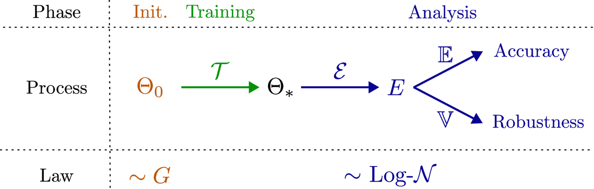
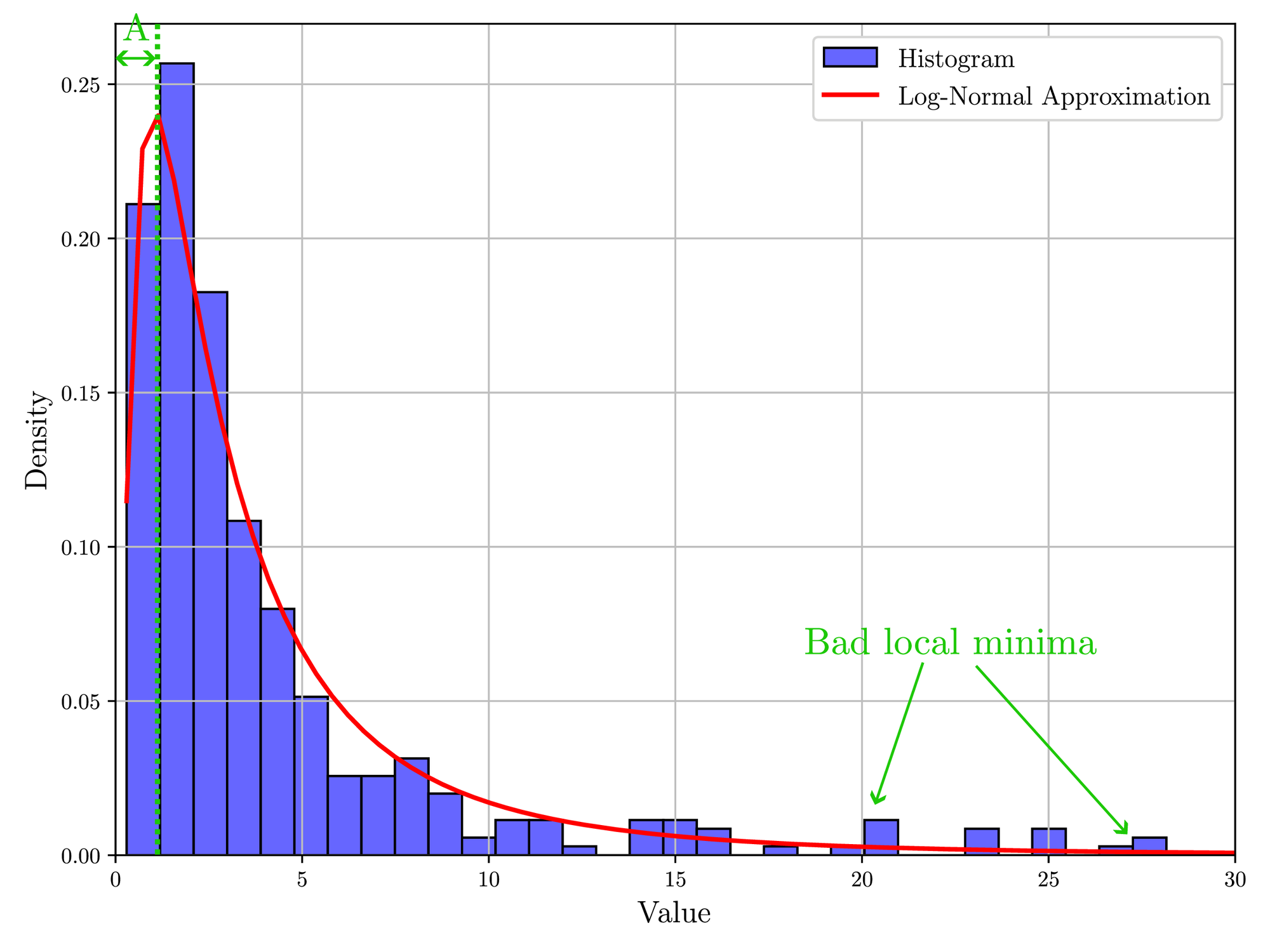
These definitions can be understood in a logical context from Figure 1. The accuracy metric is the traditional metric used to evaluate PINNs learning algorithm [24] but we want to highlight the stochasticity of the random variable \( E\) which is often neglected. The robustness metric comes from stochastic control theory [25, Chapter 6] where it is used to measure the size of the confidence interval and therefore the robustness with respect to the external parameters of the algorithm. To the best of the authors’ knowledge, this metric has not been properly studied despite its central role when characterizing the efficiency of a learning algorithm. In short, it is important to measure the accuracy of the algorithm as an indicator of how the final approximation \( v_{\Theta_*}\) is close to the real solution \( v\) and to show the approximation capabilities of the neural network. The robustness of the algorithm measures the impact of the initial condition \( \Theta_0\) on the generalization error and, consequently, shows reproducibility. A small robustness value \( R\) means that the generalization error will remain close to the accuracy, while a large value indicates that the generalization error could differ significantly for different values of \( \Theta_0\) .
For PINNs, it has been shown in [8, Theorem 7.1] and in [26] that the global minimum of \( \mathcal{L}_{\lambda}\) can be as close to \( 0\) as desired provided a sufficient number of neurons \( N\) in \( v_{\Theta}\) and Lipschitz continuity of the operator \( \mathfrak{F}\) . Moreover, in that case, the generalization error can be as close to \( 0\) as desired [8]. From the work [27], it seems that the number of local optimums increases with the number of neurons \( N\) but the local optimums tend to converge to the global optimum. In other words, these works strongly suggest that \( A(\mathcal{T})\) goes to \( 0\) with an infinite number of neurons. Since \( E = \mathcal{E}\left(\mathcal{T}(\Theta_0) \right)\) is a positive random variable, a low accuracy \( A(\mathcal{T})\) implies a small robustness metric \( R(\mathcal{T})\) . Consequently, there is evidence that indicates that \( R(\mathcal{T})\) goes to \( 0\) with the number of neurons, and then the performance of the learning algorithm would not depend on the initial condition \( \Theta_0\) .
The previous remarks explain why there has been so little interest in the robustness metric since an accurate training algorithm would naturally induce high robustness. However, in practice, the training algorithm might enter some early stopping conditions due, for instance, to saddle points, exploding or vanishing gradients [2, Section 4.3] or other PINN-specific pathologies [24]. Noise in the measurements or multi-objective problems are usually going in the opposite direction of increased accuracy. In addition, there is not an infinite number of neurons and the ecological impact of machine learning tends to justify a shallow neural network. Consequently, \( A(\mathcal{T})\) is usually strictly positive and sometimes not very small, and robustness must also be evaluated.
The last metric would relate to computational complexity. Indeed, some methods might be accurate and robust, but they require so much computational power that it is impossible to consider them in an engineering application. A rigorous evaluation of the computational complexity is tedious and, in general, very generic. An empirical measurement is the computational time and it is the one chosen in this paper.
Note that it is usually not possible to compute \( A(\mathcal{T})\) or \( R(\mathcal{T})\) and we must use estimators. However, the empirical mean and variance are very sensitive to outliers, especially with little data. Therefore, in numerical examples, we instead recommend computing the median value of \( \mathcal{E}(\mathcal{T}(\Theta_0))\) as its accuracy and its interquartile range (IQR) as its robustness measure.
As explained in [15, 24], multiple attempts have been made to derive algorithms that are more accurate for PINNs using strategies such as reformulation [8, 9], novel architectures [10, 11], new learning paradigms [12, 13] and loss reweighting [14, 15, 16]. In this paper, we focus on the latter class which consists of changing the weight \( \lambda\) during the training of (3) to improve the robustness and accuracy of the learning algorithm. That leads to the following problem.
Problem 1
We want to evaluate the robustness and accuracy of reweighting learning algorithms to estimate a solution to (1).
We also aim to propose a new strategy that is naturally supposed to ensure robustness. We decided to focus on loss reweighting because this method has much potential and is easily generalizable for rapid adoption. Therefore, we will evaluate the accuracy and robustness of loss reweighting strategies and derive a primal-dual learning algorithm that can be interpreted using traditional optimization or renowned learning techniques.
2.3 Related works
Reweighting strategies in machine learning have been investigated in multiple contexts such as classical mechanics [28], regularization [29], and multiobjective optimization [30], to cite a few. This methodology provides an interesting approach to the problem since it improves the accuracy significantly with minor modifications of the training algorithm. In the specific case of PINNs, changing the weighting during training has led to some improvements in the balancing between data and physics [15, 31]. However, a fair comparison between the different strategies with metrics is missing. In this section, we explore some of the most famous contributions made in this field.
2.3.1 The annealing method
The first paper mentioning loss reweighting as a possible strategy to improve the convergence of PINNs is [4]. To address the imbalance between the gradients corresponding to the data term \( \mathcal{L}_{\textrm{data}}\) and the gradients corresponding to the residual term \( \mathcal{L}_{\textrm{phys}}\) , they propose that the weight \( \lambda_{\textrm{data}}\) are adaptively computed utilizing the max and mean statistics of the gradients as follows:
(7)
Since the computed values are prone to considerable fluctuations, the authors performed a moving average filter. Finally, the loss was written as:
(8)
The advantage of this method lies in its simplicity. It requires very little computing power to update the weights. However, the meaning of the weights is difficult to understand. This strategy is supposed to ensure a good flow of the gradients through the network ensuring better training but there is no evidence that robustness should be increased.
2.3.2 The inverse Dirichlet weighting
Similar to the annealing method, the inverse Dirichlet weighting [32] utilizes the back-propagated gradients to adjust the weights from the data loss. Instead of calculating the maximum and average values, the authors proposed to compute the weights to prevent the gradient vanishing phenomenon based on the gradient variance as:
(9)
Then, a smoothing filter is applied as previously. The inverse Dirichlet weighing also uses the annealing loss in Equation 8. It is an uncertainty weighting method ensuring that the loss weights are inversely proportional to their respective uncertainty of the loss gradients. This method avoids then the vanishing gradient problem during the training process. However, it introduces uncertainty in the gradient flow’s direction, which can lead to convergence failure. Despite its formulation in terms of variance, nothing related to robustness is stated in [32].
2.3.3 The neural tangent kernel method
Another line of work by Wang et. al. [33] focuses on the convergence rate of different loss terms which can be examined through the Neural Tangent Kernel (NTK) during the training. The kernel \( \mathcal{K}\) is defined as:
(10)
where \( \langle \cdot, \cdot \rangle\) is the euclidean scalar product.
The authors have shown that the convergence rate of the training error is determined by the eigenvalues of \( \mathcal{K}_{vv}\) and \( \mathcal{K}_{rr}\) , and the kernel itself converges to a deterministic kernel with an infinitely small learning rate. Building on this insight, they proposed the following weight-balancing method:
(11)
where \( \text{tr}\) is the trace operator and with the loss
(12)
This method is the only one that is supported by the theory and is supposed to equalize the convergence speed of both contributions \( \mathcal{L}_{\textrm{data}}\) and \( \mathcal{L}_{\textrm{phys}}\) . However, it is very time-consuming to compute the kernels and, in the case of many physical points, it can be very slow. Moreover, equaling the convergence rates will help in balancing the two costs but it does not guarantee a more robust or accurate algorithm.
2.3.4 Other methods
There have been other more recent or elaborated methods. With an optimization perspective, the authors in [34] suggest using the celebrated Karush-Kuhn-Tucke optimal conditions to select the weighting coefficients [35, 36]. Even if this approach is successful in many linear cases, it relies on solving a secondary optimal problem, significantly increasing the training time and algorithm complexity.
Using a similar approach, recent work such as [37] suggests using augmented Lagrangian theory [38] to approximate a local optimum in a finite number of steps. This technique is widely used in classical optimization, but requires a change in the structure of the loss function and might lead to overcomplicated computations [14].
Finally, using a probability perspective with a Gaussian likelihood, the authors in [39] provided a new framework to increase contributions that do not follow a Gaussian error with prescribed parameters. This interesting approach assumes normal behavior and requires a more complex loss function.
In the same vein, but with a different objective in mind, the authors in [16] propose using causality to design the weight and increase the importance of the losses as time increases. The suggested method proposes a solution for dynamical systems that have a time dependence. We are not investigating it here, since it refers to a more specific class of systems.
Concerning the stopping criteria, the original papers use the L-BFGS solver [40] which naturally includes early stopping conditions such as limited evolution or insactisfaction of the Wolfe conditions [41]. In modern optimization, it becomes more and more common to use the PL-condition [42, 43] which relates to a significant decrease of the loss function compared to its gradient. However, all these stopping criteria are not associated with PINNs and their specific behavior, which is to approximate a function knowing its dynamical properties.
3 A robust by design method: The Primal-Dual algorithm
The primal-dual method is used in optimization to provide an approximation to NP-hard problems [44]. The idea is to rephrase the original problem into two different and complementary sub-problems, primal and dual, which can be solved simultaneously, leading to Algorithm 1.
Algorithm 1 Primal-Dual (PD) algorithm for (13).
Hyperparameters: \( \varepsilon\) , \( \alpha_{\Theta}\) , \( \alpha_{\lambda}\) , \( D_{\textrm{test}}\) , \( N_{\lambda}\) , \( N_{\Gamma}\) , \( N_{U}\) , \( N_{\textrm{epoch}}\) , \( N_{\textrm{resample}}\) .
Algorithm 2 Function stopping_criterium: Stopping criterium for PINN problem (4).
Before explaining the reasons behind this algorithm, we can first note that the instructions written in black are similar to the vanilla PINN’s training with a first-order method (in particular the gradient descent update on line \( 11\) ). This paper is introducing two novelties: 1) the dual update (gradient ascent) on line \( 13\) (in green), and the stopping condition on lines \( 5-7\) (in red). These minor modifications make the overall additions easy to implement on a vanilla PINN. The stopping criterion was added to compare different algorithms’ convergence rates and computational complexity. We show in the following proposition that the stopping criterion will terminate the algorithm if sufficient accuracy and robustness are obtained.
Proposition 2
Let \( N_{\textrm{epoch}} = \infty\) , and
Assume that both \( f\) and \( g\) are \( L\) -gradient Lipschitz with
and \( D_{\textrm{test}} = D_U\) with no resampling in \( \Gamma\) and \( U\) .
If there are enough neurons then Algorithm 1 terminates almost surely at step \( k_*(\varepsilon)\) for any \( \varepsilon > 0\) and \( \lim_{\varepsilon \to 0} g(\Theta_{k_*(\varepsilon)}) = 0\) .
The proof is available in B.
Remark 2
Note that we did not use the condition on \( \| \nabla_{\Theta} \mathcal{L}_{\lambda_*}(\Theta_*, D_\Gamma, D_U) \|\) to terminate the algorithm. The reason is that \( g\) is very noisy because of the numerical derivation and the noninfinitesimal step. However, the function \( e_k\) (Algorithm 2, line \( 2\) ) does not depend explicitly on \( g\) and is, therefore, a better criterion to terminate the algorithm. It is also a more interpretable measure because we are interested in a convergence of the function and not of its weights. \( \square\)
Remark 3
The current version of the stopping criterium is robust since it is working on an average (\( C\) in the proof) of the error metric \( e\) . However, to avoid early stops, it can be made even more robust by considering it to be verified on multiple consecutive samplings, meaning that \( \mathfrak{F}[v_{\Theta_*}]\) is closer to \( 0\) on \( U\) . \( \square\)
The assumptions made in the previous propositions are relatively strong but true, at least locally, in practice [8]. Moreover, the resampling has been neglected to simplify the mathematical derivation but it is possible to include it. The previous proposition does not ensure that \( f(\Theta_*) = 0\) , in other words, there is no guarantee that Algorithm 1 converges to the global minimum. However, it almost always converges to \( g = 0\) , no matter the initialization \( \Theta_0\) . Under Assumption 1 and the existence of a unique solution, this is a robustness result. In the following subsections, we propose to justify this algorithm using an optimization perspective and then a learning viewpoint.
3.1 The Primal-Dual method from an optimization perspective
Approximating a weak solution \( v\) to the original problem (1) is equivalent to solving the following one on \( v_{\Theta}\) :
(13)
Remark 4
Note that in this formulation, we write that satisfying the PDE is a hard constraint, fitting the measurements being left as a secondary objective. That means that, in the case of an incompatibility between the PDE and the measurements, we prioritize satisfying the PDE over the measurements. This can be particularly impactful in the case of high-frequency boundary values \( v_{\Gamma}\) where high orders might be neglected to prioritize the solution of the PDE. \( \square\)
The Lagrangian [38] related to the previous system is defined as
(14)
with \( \lambda > 0\) . Following the Lagrangian theory, the constrained optimization problem defined in (13) can be relaxed to the following unconstrained \( \min\) -\( \max\) problem:
(15)
The primal-dual approach consists in solving these two problems:
(16)
and
(17)
Instead of solving a sequence of primal-dual problems as proposed in [38], the main idea is to alternate between solving the primal and the dual to get close to a local optimum of the original constrained problem [44]. This methodology has been investigated in other settings by the authors of [45, 46] who considered solving these two problems in parallel to decrease training time.
Basically, problems (16)-(17) are not numerically tractable since they contain integrals. An approach consists of using Monte-Carlo approximations as follows:
(18)
where \( D_{\Gamma} \subset \Gamma\) and \( D_{U} \subset U\) are finite sets. If we denote by \( N_{\Gamma}\) and \( N_U\) the number of points in \( D_\Gamma\) and \( D_U\) respectively, the law of large numbers ensures that if the sets \( D_{\Gamma}\) and \( D_{U}\) are uniformly sampled from \( \Gamma\) and \( U\) , both with volume \( 1\) , then
A numerically tractable relaxed version becomes
(19)
and
(20)
Since \( \nabla_{\lambda} \mathcal{L}_{\lambda}(\Theta) = g(\Theta)\) , the gradient-ascent from equation (20) translates to the instruction in line \( 13\) of Algorithm 1. Consequently, the primal-dual method applied to (19) and (20) leads to Algorithm 1.
3.2 The Primal-Dual method from other perspectives
The previous subsection justified the use of Algorithm 1 and Proposition 2 ensured convergence in the limit case. We propose here to take other perspectives and justify Algorithm 1 using robustness arguments.

3.2.1 Adversarial learning perspective
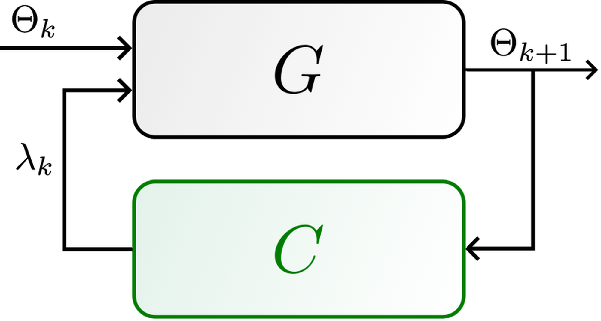
In the optimization form (15), it appears clearly that the objective of the learning algorithm is to learn among all possible solutions to the data, the only one that also solves the residual. Then it fits the framework of generative adversarial learning [47]. The neural network will generate a possible solution to the data through the primal update (system \( G\) in 4) while the discriminator (system \( C\) in 4) will discard solutions that violate the physics of the system by increasing the physics loss (dual update).
Training a generative adversarial network follows an algorithm similar to Algorithm 1 (see Algorithm 1 from [47]) at the difference that the discriminator is updated more frequently than the generator. These models are known to be often more accurate but also more robust [48] since the discriminator will penalize solutions that are not suitable. Using control terminology, the open-loop system in Figure 3 is less robust (and maybe even unstable), while the closed-loop one in Figure 4 is supposed to have better convergence properties if the design of \( C\) is successful. This is ensured through Proposition 2 which guarantees \( g(\Theta_*) = 0\) if \( \alpha_{\lambda}\) is sufficiently small and provided enough neurons.
Note that resampling is also part of the discriminator since we want to have a low residual throughout the whole domain and, therefore, the empirical Lagrangian \( \mathcal{L}_{\lambda_*}(\Theta_*, D_{\Gamma}, D_U)\) should be low for any \( D_\Gamma\) and \( D_U\) . Indeed, it appears clearly that if \( \int_U \| \mathfrak{F}[v_{\Theta_*}] \|^2 = 0\) , then necessarily \( g(\Theta_*) = 0\) for any sampling \( D_U\) . This implies that any local minimum of the Lagrangian \( \mathcal{L}_{\lambda}\) as in (14) is also a local minimum of the empirical Lagrangian \( \mathcal{L}_{\lambda}(\cdot,D_{\Gamma},D_U)\) for any sampling \( D_{\Gamma}\) and \( D_U\) . The reverse is not true but we can claim that if a local minimum is shared across multiple samplings then the probability that it is also a local minimum of the real Lagrangian is high.
Resampling can then be seen as an adversarial strategy since, as soon as the physics residual is small, a new sampling will most probably increase the loss. This remark is shedding light on the parameter \( N_{\lambda}\) which relates to the frequency of the dual update and the resampling. Indeed, if we resample too often, then the gradient descent update will not get enough time to reach a local minimum on this sampling. This might result in undesirable oscillations of the loss. On the contrary, if \( N_{\lambda}\) is too large the stopping criterion might stop the algorithm too early while, on some other samplings, the empirical loss might still be large. Both cases can be diagnosed easily from the loss plot along epochs.
3.2.2 Curriculum learning perspective
Curriculum learning is a type of learning that has been investigated since 2009 in [49]. The idea is that training a complex model from scratch might be challenging. Instead, if one can divide the learning problem into several simpler tasks of increasing difficulty, learning from the previous optimum should lead to better convergence. This has been mathematically phrased as the entropy of the training distribution should be increasing during the training and reach, in the end, the real entropy.
In [50], for example, it has been shown that the entropy is actually related to the loss landscape. The loss landscape represents the variation of the loss when the parameters \( \Theta\) are moving continuously in some interval. Assuming that the loss is differentiable, the entropy is then related to the Hessian of the loss \( \mathcal{L}_{\lambda}\) [51]. In the case of PINNs, the loss landscape has been investigated in [5, Section 5] and the conclusion is that the physics loss \( \frac{\lambda}{\left| D_{U} \right|} \sum_{u \in D_{U}} \left\| \mathfrak{F}(u) \right\|^2\) contributes the most to the entropy of \( \mathcal{L}_{\lambda}\) . Consequently, following a curriculum learning strategy, it seems better to start with \( \lambda = 0\) to obtain the minimum entropy and then increase it during training to reach, in the ideal case, \( \lambda = \infty\) . However, quite often, a local minimum is reached for \( 0 < \lambda < \infty\) which will stop training.
The aim of Algorithm 1 is then to avoid getting stuck at a local minimum that is far from a global one of the residual. To that extent, the cost is modified during the training. Moreover, the updates of the cost are made in such a manner that the constraint should be enforced at the limit.
3.3 Primal-Dual as a pretraining
Even if Algorithm 1 works well in theory, it is, however, slow and tends to oscillate around the local optimum (as any first-order optimization scheme [2, Section 8.5]). A second-order solver is usually faster and does not oscillate as much at the end of the training [2, Section 8.6.1]. However, changing the cost during the training is not straightforward, implying that it is more sensitive to initialization and ill-conditioning.
An idea is to combine the advantages of both solvers by using a first-order method as a pretraining with a limited number of epochs. Since gradient descent algorithms have a convergence rate of \( 1/k\) with \( k\) the number of epochs [52], we get that \( e_k\) is decreasing fast in the first epochs. Bad local minima around the initialization are thus avoided. Using a second-order solver with the warm startup \( \Theta_k\) obtained from the first-order solver enables faster convergence, with increased robustness.
4 Numerical simulations and discussion
In this section, we conduct a collection of comprehensive numerical simulations in order to assess the performance and robustness of the proposed Primal-Dual algorithm against the other state-of-the-art training methodologies to solve PDEs. To facilitate a direct comparison with those established methodologies presented in the original paper, we employ the same loss function they described, despite potentially leading to a different interpretation of the loss and weights. Section 2.3 describes the meaning in each specific case. To enable a good comparison, we normalized all results with the median of the L-BFGS accuracy (original PINN’s training strategy). Note that we also implemented pure ADAM [53] with fixed weights to compare if the balancing algorithms improved the first-order method. Finally, to check that the way the weights \( \lambda\) are updated matters, we also compared with a random evolution (ADAM-Random).
In the following sections, the results obtained from three different PDEs are gathered. The parameters for the algorithms are kept the same as in their original article except for the resampling rate \( N_{\textrm{resample}}\) and dual update rate \( N_{\lambda}\) which are always set to every \( 500\) and \( 50\) iterations of gradient descent respectively except for NTK where the dual update rate \( N_{\lambda}\) remains at 500 as specified in the original paper. In particular, the batch size of the sampling and the neural network structure are tailored to the complexity of each equation. The accuracy and robustness metric is evaluated for the performance of algorithms as described in Section 2.
The codes are written in Python using Tensorflow 2 and all the results are obtained on KTH EECS online GPU services with a 20 GB shared GPU of NVIDIA DGX H100. The code is available on GitHub.
We first describe the three cases studied and report the corresponding results. Then we discuss these outcomes.
4.1 Case studies definition
4.1.1 Case study 1: one-dimensional quasi-linear hyperbolic equation
To show the ability to solve time-dependent problems, the first example comes from the traffic state estimation problem [54], which is the simplest macroscopic model of traffic flow and considers the following viscous Burgers’ equation [55]:
(21)
where \( \rho \in [0, 1]\) is the normalized density of vehicles, and \( V_f > 0\) is the free flow velocity. We are interested in the case where we approximate the solution to the hyperbolic problem (\( \gamma = 0\) ), and we therefore select a very small viscosity \( \gamma\) .
The simulation results are obtained with the following initial and boundary conditions:
(22)
where \( \rho_1, \rho_2, \rho_3 \in [0, 1]\) are drawn randomly between \( 0\) and \( 1\) . These conditions simulate all kinds of Riemann problems: a shock (discontinuity) or a rarefaction (smooth transition). Since the initial condition is a simple function with three components, all kinds of phenomena might appear and also interfere, leading to a more complex shape. In the case \( \gamma = 0\) , there might be multiple solutions. However, only one is meaningful and is called the entropic solution. It corresponds to the limit when \( \gamma \to 0\) of (21). With this setup, we want to evaluate if the algorithm manages to extract the entropic solution or if it will converge inaccurately to the non-entropic one.
To compute the accuracy of the method, the solution to (21) is approximated using a finite difference numerical scheme. The stability and consistency of the numerical scheme are ensured through the CFL condition [56]. For this problem, the simplicity of the analytical solution suggests sampling with \( N_\Gamma = 2520\) and \( N_U = 3000\) , and using a simple neural network such as a 2-hidden-layer fully connected network with \( 10\) and \( 5\) neurons per layer.
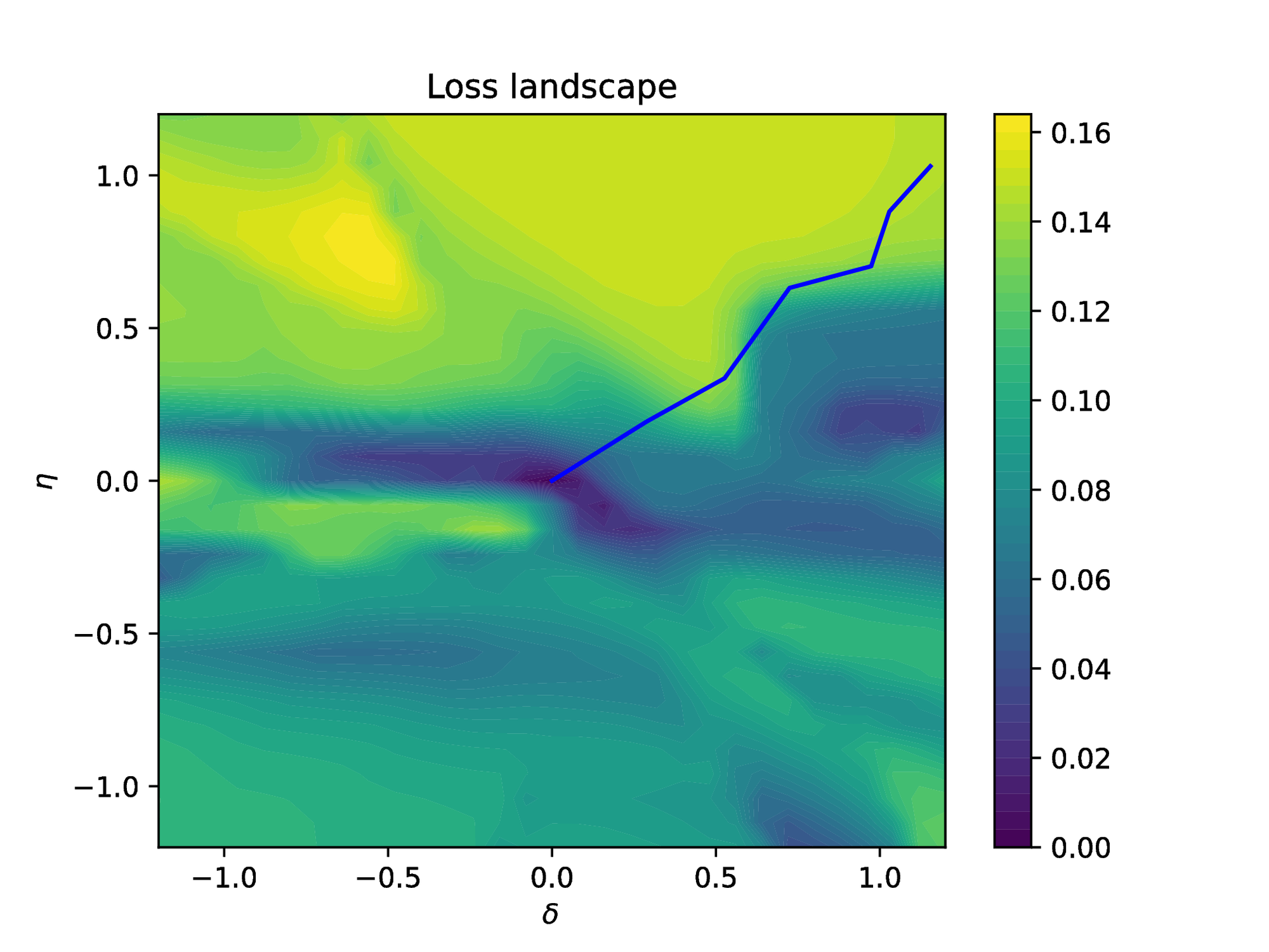
We ran the seven described algorithms with and without pretraining (when meaningful) on this model. To get statistically significant results, we ran each algorithm \( 30\) times with different initial tensor parameters \( \Theta_0\) . To enable a fair comparison, all algorithms are using the same random initial and boundary conditions (22). The results are reported in Figure 5. For a better understanding of the Primal-Dual algorithm, the final loss landscape is plotted in Figure 8. In this figure, the blue line represents the trajectories of the loss during the training.
4.1.2 Case study 2:
The second example, the Helmholtz equation, demonstrates the ability to solve time-independent problems, which has been widely studied in many areas of physics such as acoustics and electromagnetics [57]. We consider the following two-dimension Helmholtz equation:
(23)
given a source term of the form:
(24)
One can easily derive the exact solution to this equation as: \( u(x,y) = \sin{\pi x} \cdot \sin{4\pi y}\) . This example is taken from [4] since it has been shown rather difficult to learn because of the source term. We considered a \( 3\) -hidden-layer neural network with \( 50\) , \( 50\) , and \( 20\) neurons per layer for this problem. The training data are sampled with \( N_\Gamma = 400\) and \( N_U = 500\) points.
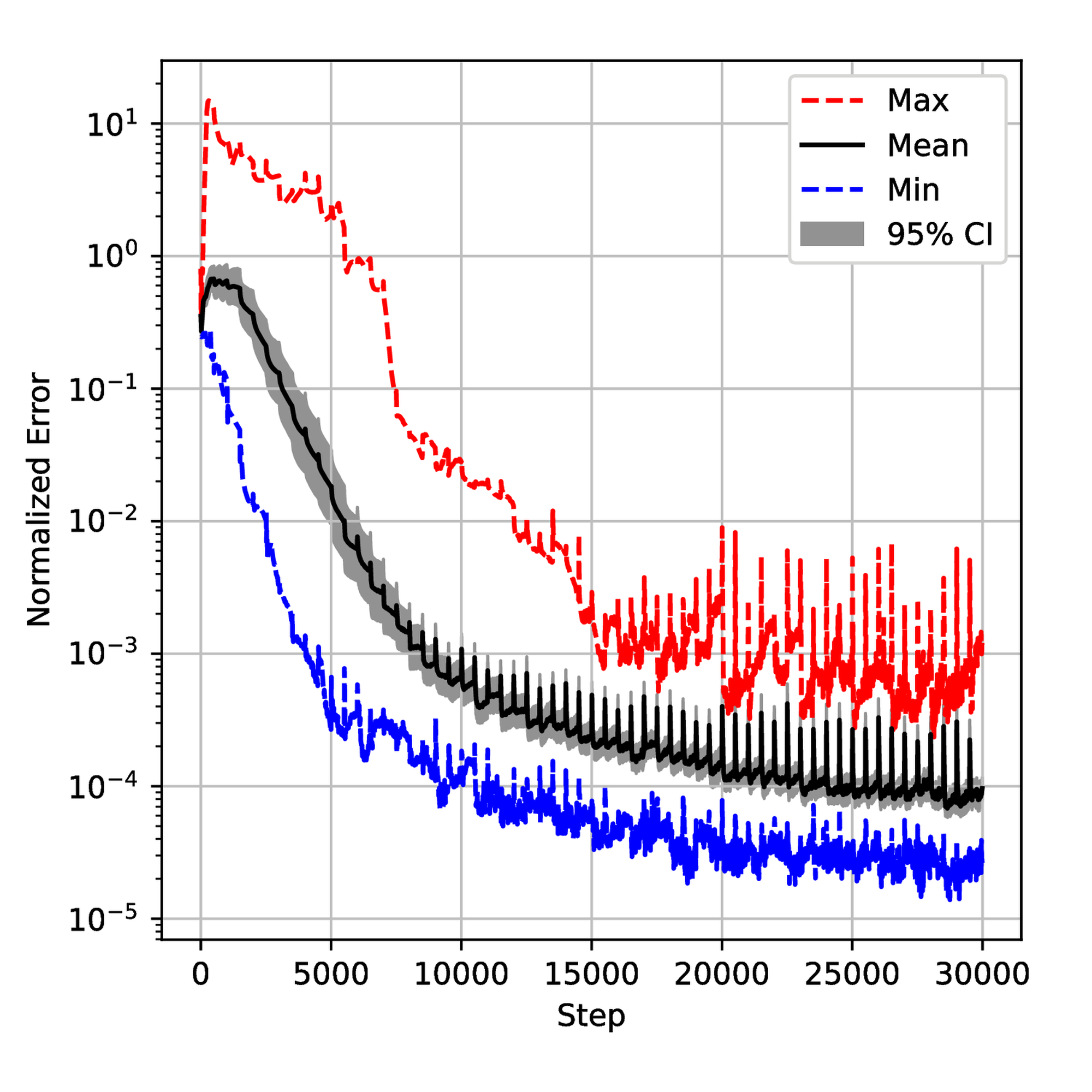
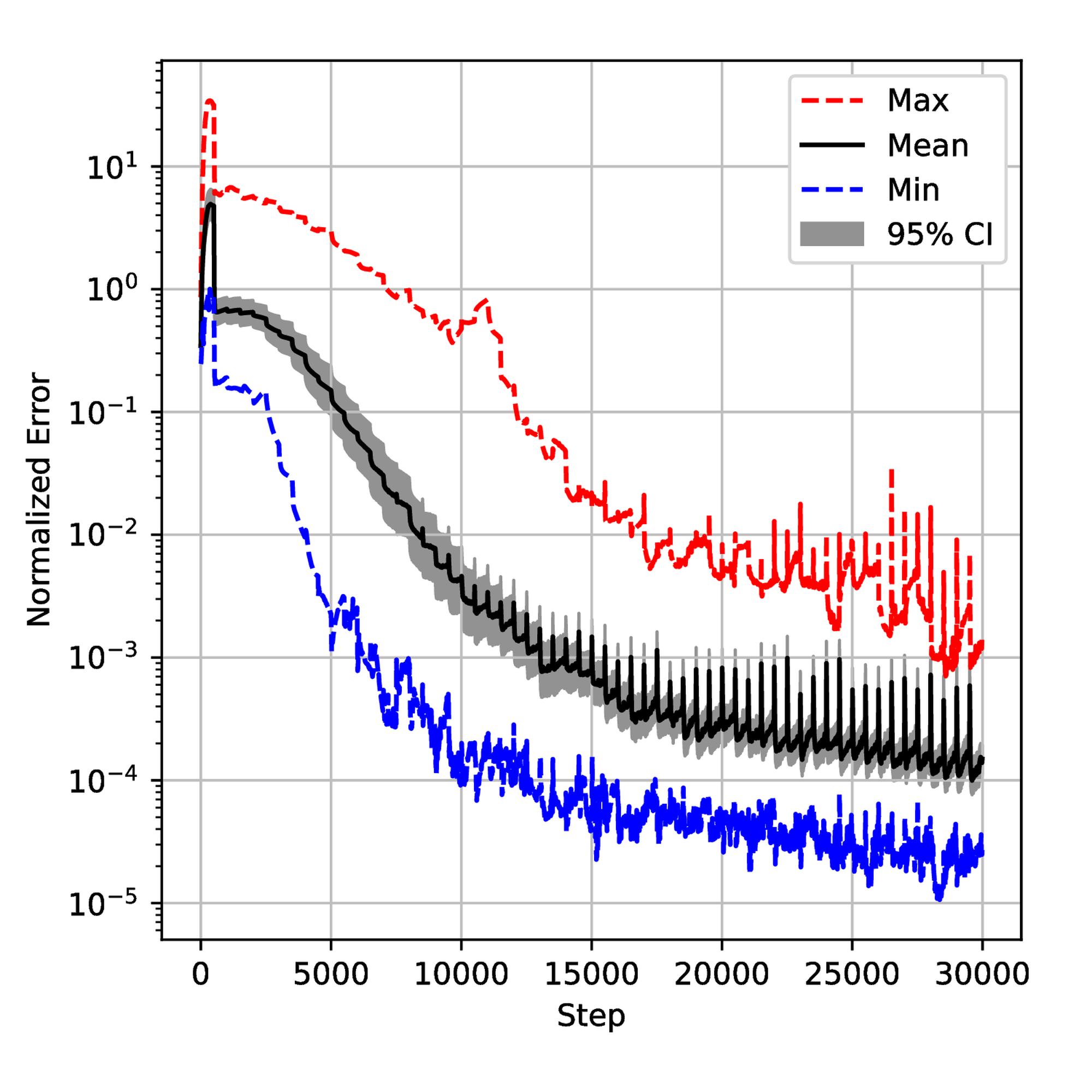
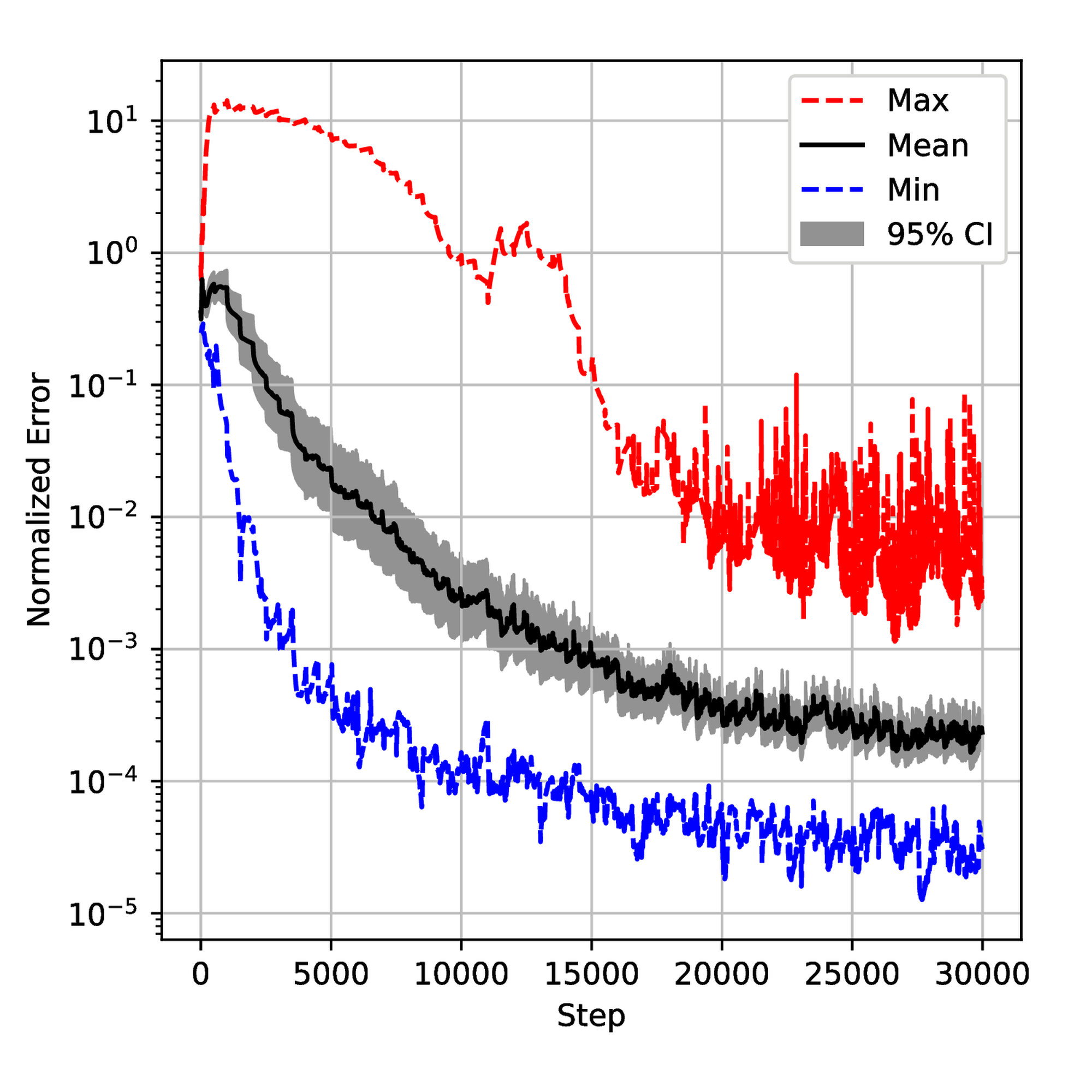
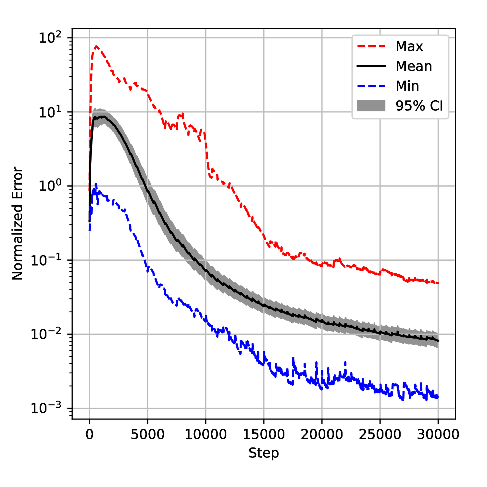
The seven described algorithms with and without pretraining were employed to solve this problem. Similar to the first example, we executed each algorithm \( 20\) times with different initial tensor parameters \( \Theta_0\) and sampling seeds to ensure the significance of the statistical results. The results are shown in Figure 9. Meanwhile, we monitored the evolution of the weight \( \lambda\) and the generalization error during the training process for each algorithm. The results are displayed in Figure 12 and Figure 18 respectively. We also gathered results from all simulations and normalized them to get the normalized histogram of the random variable \( E\) (generalization error) from equation (6) in Figure 23.
4.1.3 Case study 3:
The 1D Poisson equation is a fundamental partial differential equation that describes the distribution of a scalar quantity, such as potential or temperature, influenced by a source term in a one-dimensional domain. The general form of the equation is given as:
where \( \Delta\) is the Laplace operator, \( u\) is the unknown solution and \( f\) represents a known source term that introduces excitation. In this case study, we examine the following 1D Poisson’s equation:
(25)
where the solution is \( u(x) = \sin{0.7x} + \cos{1.5x} - 0.1x\) . We sampled \( N_\Gamma = 2\) and \( N_U = 400\) points randomly in \( U\) and the network contains \( 2\) hidden layers with \( 30\) neurons per layer. The comparison between the algorithms is available in Figure 24.
4.2 Discussion
4.2.1 Observation
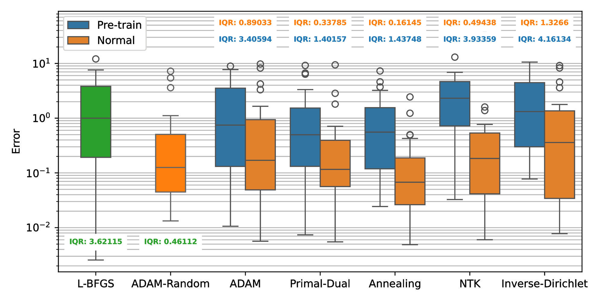
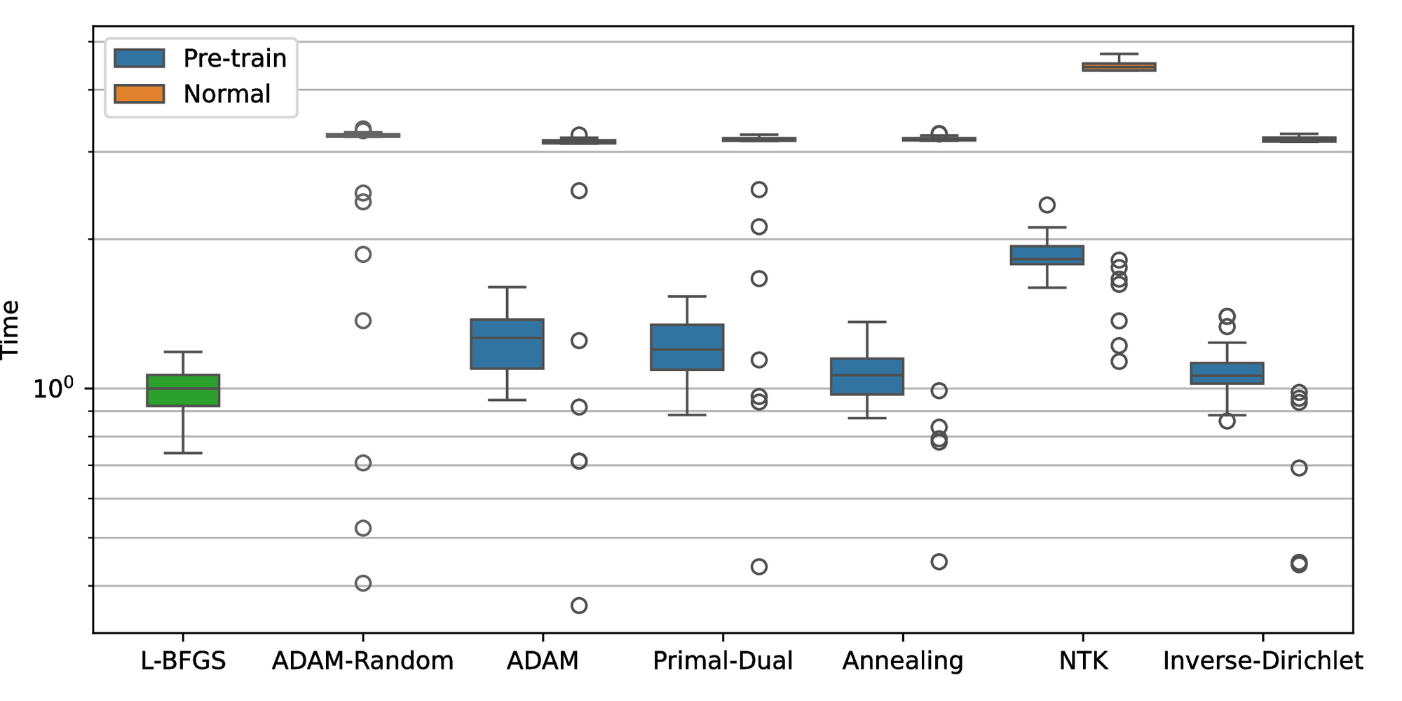
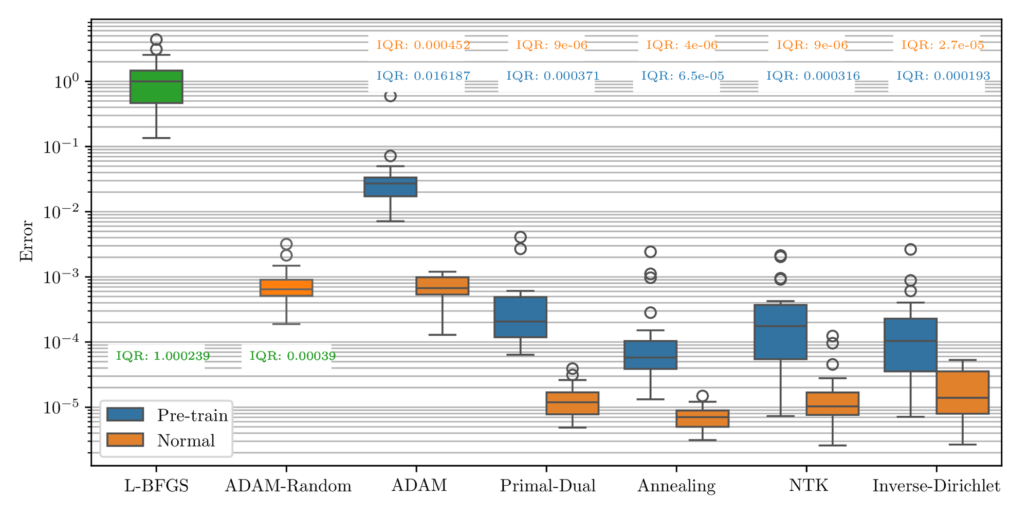
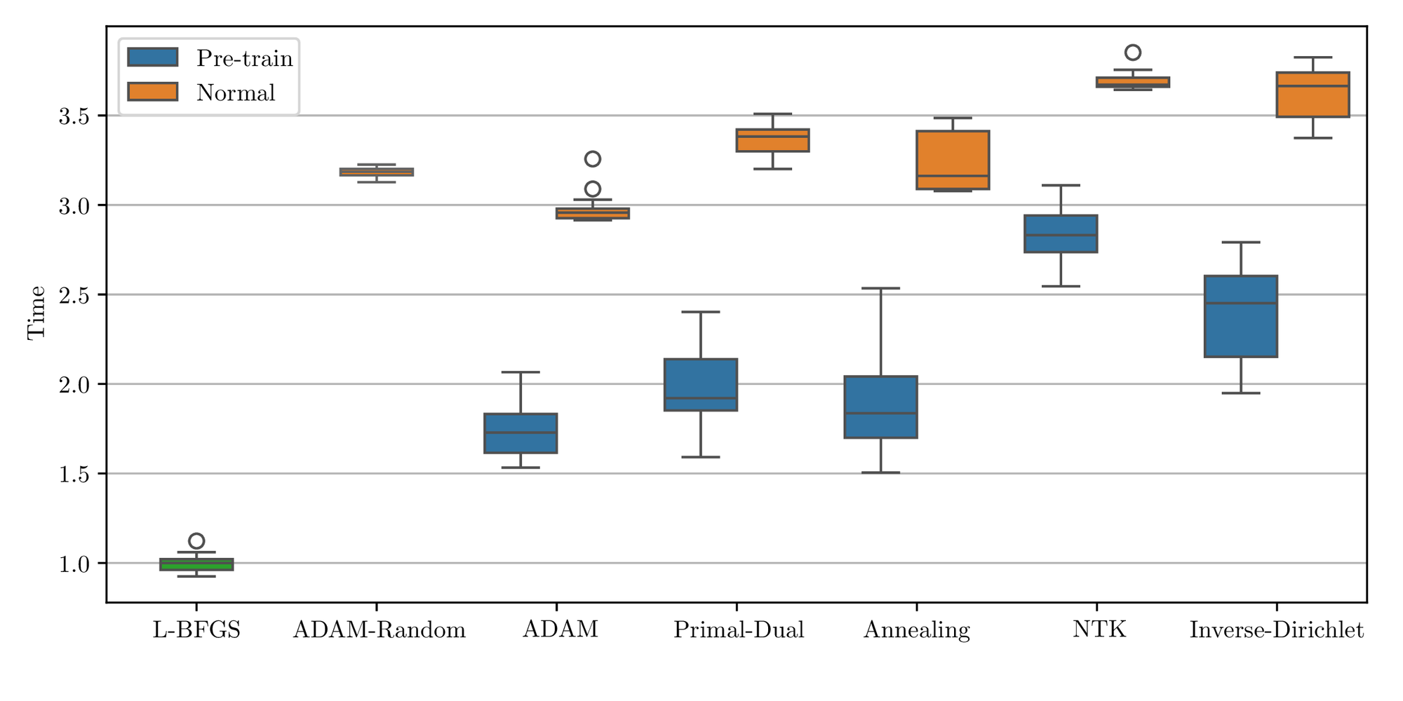
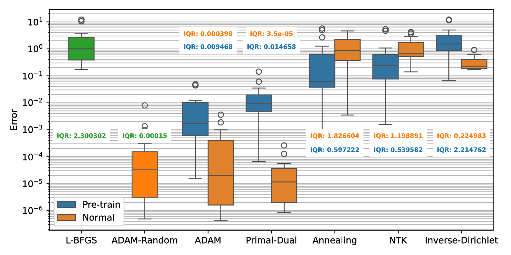
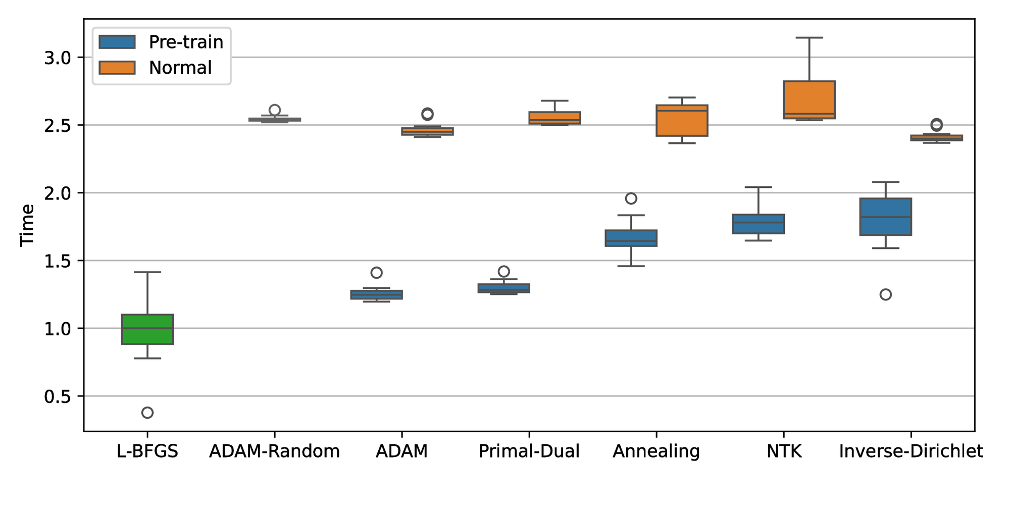
In the first case study, the error plot in Figure 6 shows that all weight-balancing methods improve the accuracy compared to the L-BFGS algorithm. The annealing method obtains the lowest median error and IQR among algorithms, which is around 20 times lower than L-BFGS. Primal-Dual and ADAM-Random achieve the second smallest median error but the former shows a slightly lower IQR. Meanwhile, ADAM and NTK show nearly identical median error but the NTK’s IQR is approximately 80% of the ADAM’s. Inverse-Dirichlet, however, exhibits a significantly higher median error and IQR compared to other weight-balancing methods. For the pretraining cases, ADAM, Primal-Dual, and Annealing all improve accuracy and robustness, whereas NTK and Inverse-Dirichlet methods perform worse than the L-BFGS only. When it comes to computational time, Figure 7 indicates that all weight-balancing methods are approximately 3-4 times more costly than L-BFGS, whereas pretraining significantly reduces the time cost.
Figure 10 shows that the weight-balancing methods achieve similar optimal results compared to the baseline for the second study case. ADAM and ADAM-Random are nearly identical with a median error of around \( 7\times10^{-4}\) and an IQR on the order of \( 10^{-4}\) . The Annealing method demonstrates the best result with the smallest median and IQR values. In contrast, the Primal-Dual and NTK methods show nearly identical median, which are slightly higher but comparable with the Annealing method. Although the Inverse-Dirichlet method performs better than the baseline algorithms and has a similar median error as the others, it has a relatively larger IQR value. Similar to the normal-training cases, the Annealing method with pretraining continues to demonstrate the best performance, achieving the smallest median \( 5\times10^{-5}\) . The Primal-Dual and NTK methods with pretraining demonstrate comparable performance with the median error and IQR values around \( 10^{-4}\) . Although all pretraining algorithms exhibited better results compared to L-BFGS, they performed worse than the normal training in this problem. Figure 11 presents the computational time for each algorithm. The algorithms with normal training exhibited similar trends to those observed in the first example, with a computational time around \( 3-4\) times higher than L-BFGS. ADAM is the fastest algorithm among all algorithms followed by the Annealing method, Primal-Dual, Inverse-Dirichlet, and NTK with normalized median values of 3.2, 3.4, 3.6, and 3.7 respectively.
The error plot for the third case (1D-Poisson equation) in Figure 25 shows that the ADAM-Random and ADAM exhibit similar performance to the first two cases, with significantly lower median error compared to L-BFGS. Although ADAM shows a better median (twice as good) in this case, its IQR is more than twice that of ADAM-Random. Primal-Dual shows its effectiveness in this case, with a median error that is twice smaller than ADAM’s and the lowest IQR at \( 3.5 \times 10^{-5}\) . However, the other weight-balancing methods (Annealing, NTK, and Inverse-Dirichlet), perform much worse in this example. While the NTK and Inverse-Dirichlet still outperform L-BFGS, with approximately twice and 5 times lower the median, respectively, the Annealing performs almost the same as L-BFGS. In the pretraining cases, Annealing and NTK do not perform as well as ADAM and ADAM-Random methods but show improvement compared to normal training. When it comes to computational time, all the normal training algorithms show a similar cost of 2.5 units in Figure 26. ADAM and Primal-Dual with pretraining successfully decrease the time cost to approximately \( 1.2\) units time spent, while the other pretraining algorithms decrease the average time spent to \( 1.5-2\) units.
4.2.2 Interpretation
In the first case, the results of ADAM and ADAM-Random indicate that changing \( \lambda\) during the training process indeed improves the performance of the algorithm. Meanwhile, the results of Primal-Dual and NTK are also quite close to ADAM-Random. In that example, the way we change the weights seems to have a minor influence on the generalization error. This might be due to the simple structure of the neural network, which limits its ability to approximate the solution from the data effectively. This might also lead to the worse performance of Inverse-Dirichlet as it computes the variance of the gradients but in this case, the gradients can be very noisy.
The loss landscape in Figure 8 shows that the local minimum for \( \delta = 1\) and \( \eta = 0.2\) has been avoided by the primal-dual method even if it would have probably been targeted by the standard gradient descent algorithm. This shows that weight-balancing methods are efficient solutions for escaping bad local minima ensuring convergence to better ones.
For the second example, as the increase of complexity of neural network layers, the results of weight-balancing methods all outperform the baseline algorithms. In this case, updating \( \lambda\) randomly achieves a similar median but slightly decreased IQR, indicating that the way we update \( \lambda\) actually matters. Although the performance of weight-balancing methods are close, it is not surprising to see that Inverse-Dirichlet method achieves hightest median and IQR in this example. Using the variance of the gradients would introduce an unexpected influence on the update policy. In addition, the NTK method requires the most computational time because it deals with a matrix whose size is linearly dependent on the number of samples.
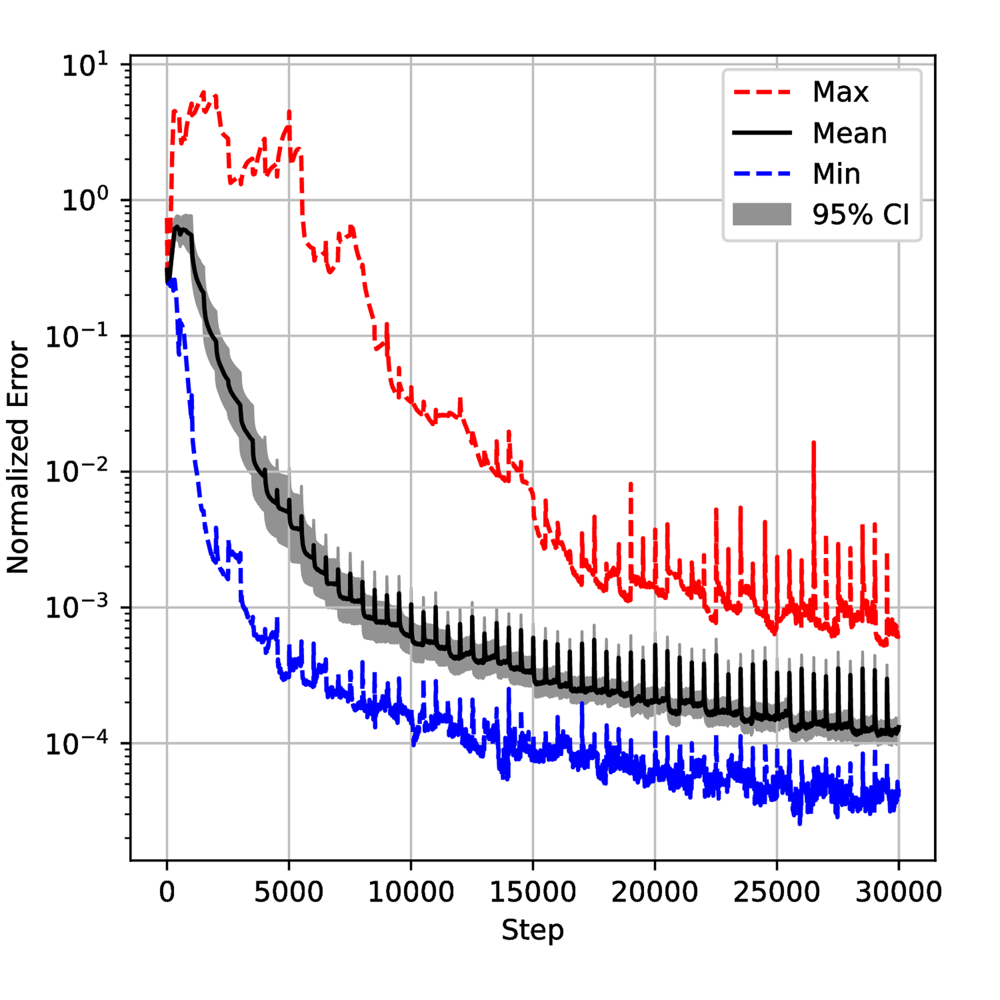
To understand the training process deeply, we saved the normalized error on test data sets and \( \lambda\) during the training for 50 runs and then plotted confidential intervals for each step. The results are displayed in Figures 12 and 18. One can observe small spikes in Figures 13, 14, and 15 which are caused by the resampling. Although all the error evolutions have a similar trend, the Primal-Dual and Annealing are significantly faster. By step \( 10,000\) , the mean error for both methods is below \( 10^{-3}\) which is 10 times lower than NTK and Inverse-Dirichlet and 100 times lower than ADAM. They also exhibit a lower variance, showing that they must lead to a more robust training.
Despite the \( \lambda\) being defined differently in each method, Figure 18 provides some insights. As shown in Figure 19, the Primal-Dual method shows a relatively fast convergence and stability with the mean value converging around step 5000. In contrast, the Annealing method converges more slowly and is less smooth than the Primal-Dual method. The NTK method exhibits a large overshoot, as seen in Figure 21. The Inverse-Dirichlet method shows the highest oscillations in this case (see Figure 22).
The histogram in Figure 23 shows that the generalized error (eq. (6)) seems to follow a Log-Normal distribution. This is logical since a very low generalization error is highly improbable as the neural network will not be able to fit the exact solution perfectly. Consequently, \( A\) is related to the number of neurons (Proposition 1). Similarly, a high generalization error would mean a convergence to a bad local minimum, which has been shown to be less probable with increasing neural network size [27]. The purpose of a "good" training algorithm \( \mathcal{T}\) is then to decrease the tail and not especially to reduce \( A\) , which related to a lower robustness value \( \mathcal{R}(\mathcal{T}))\) .
The Primal-Dual method’s results may stem from its balanced approach to adjusting \( \lambda\) , enabling to quickly find an optimal path while the overshoot in the NTK method might be influenced by the small sample size and its resampling strategy. In contrast, the Annealing and Inverse-Dirichlet methods update \( \lambda\) through the network parameters gradients, which can be biased and uncertain for each sample. Although they both implement a moving average filter, it could be difficult the choose the hyperparameters in the filter.
The failure of the Annealing, NTK, and Inverse-Dirichlet methods in the third example might be due to the imbalance of the sampling size. We observe that the boundary loss in these methods converges to zeros in the first several dual update periods and the corresponding \( \lambda\) diverges during the training.
4.2.3 Conclusion
Through three study cases, we showed that Primal-Dual exhibits more consistent improvements across different scenarios. While the Annealing method outperforms in most cases, it is not universally effective due to factors like sampling sizes. Meanwhile, it seems that NTK and Inverse-Dirichlet methods would not only be affected by the sampling sizes but also the structure of the neural networks which leads to more tuning in the hyperparameters. In conclusion, given its easy implementation and robust outcomes, the Primal-Dual method is recommended as the preferred choice. The Annealing method can be employed if one wants to obtain better results at the price of more hyperparameter tuning for a consistent behavior.
5 Conclusion
The accuracy, robustness, and computational complexity of a learning algorithm are critical factors in selecting the most suitable approach. PINNs are particularly sensitive to the initialization of neural network parameters, making robustness a key concern—especially when comparisons with alternative methods are not feasible. This study introduced a mathematical framework to define and evaluate the robustness and accuracy of learning algorithms. A novel robust-by-design approach based on the primal-dual optimization method was proposed and benchmarked against classical weight-balancing techniques for training PINNs. Numerical experiments demonstrated that while vanilla PINNs can sometimes achieve high accuracy, they often lack robustness. Weight-balancing methods emerged as efficient and accessible solutions for improving robustness. Notably, while the primal-dual method was not always the most accurate, it consistently delivered reliable results across all three case studies.
This work provides practitioners with a clear comparison of existing algorithms, highlighting that while the annealing method is the most accurate, the Primal-Dual approach is the most consistent and robust. The versatility of the Primal-Dual formulation makes it a promising candidate for further development. Future work will focus on generalizing its application to more complex domains with more competitive costs.
Acknowledgments
The authors acknowledge Elis Stefansson and Karl Henrik Johansson for their interesting discussions and proofreading.
A Proof of Proposition 1
The proof is highly inspired by [8, Theorem 7.1] or the simpler [58, Theorem 1, extended version].
From Assumption 1, let \( v\) be a solution in \( \mathcal{H}\) to \( \mathfrak{F} = 0\) with \( v = v_{\Gamma}\) on \( \Gamma\) . Since \( v_{\Theta} \in \mathcal{C}^{\infty}(U, \mathbb{R}^p) \subset \mathcal{H}\) , we get:
(26)
Using Assumption 2 about Lipschitz continuity of \( \mathfrak{F}\) , there exists \( C > 0\) such that:
(27)
For \( v \in \mathcal{H}\) , denote by \( D(v)\) the set of all meaningful weak-partial derivatives of \( v\) . Since both \( v, v_{\Theta} \in \mathcal{H}\) , Theorem 3 by [59] holds implying
Injecting the previous inequality in (27) and considering that \( U\) is bounded leads to
The constant \( K\) depends on \( \lambda\) , \( C\) and the geometry of \( U\) .
B Proof of Proposition 2
Using Theorem 2.2 from [60], under the conditions of the proposition, we get almost surely that
(28)
Note that \( v_{\Theta}\) , as defined in (2) is locally Lipschitz continuous in the parameters. Specifically, one can write for all \( u \in U\)
From (28), there exists \( K_1 > 0\) such that for all \( k > K_1\) , \( \| \Theta_k - \Theta_* \| < \theta\) . After a primal update, one gets for all \( u \in U\) :
(29)
Let, for \( i \in \{k_*-N_{\textrm{resample}}, \dots, k_*\}\) and \( k_* \mod \xi N_{\textrm{resample}} = 0\) :
Using the inequality (29) leads to:
and then
From (28), we get for any \( \varepsilon > 0\) , there exists \( K_2 > K_1\) such that for all \( k > K_2\) , we get
leading to \( C(k) \leq \varepsilon\) and the algorithm terminates.
References
[1] Physics-informed neural networks: A deep learning framework for solving forward and inverse problems involving nonlinear partial differential equations Journal of Computational Physics 2019 378 686–707
[2] Deep Learning MIT Press 2016
[3] Understanding the difficulty of training deep feedforward neural networks Proceedings of the thirteenth international conference on artificial intelligence and statistics 2010 249–256 JMLR Workshop and Conference Proceedings
[4] Understanding and mitigating gradient pathologies in physics-informed neural networks SIAM Journal on Scientific Computing 2021 43 5 A3055-A3081
[5] Challenges in training PINNs: A loss landscape perspective arXiv preprint arXiv:2402.01868 2024
[6] Pre-training strategy for solving evolution equations based on physics-informed neural networks Journal of Computational Physics 2023 489 112258
[7] MILP arXiv preprint arXiv:2501.16153 2025
[8] DGM Journal of computational physics 2018 375 1339–1364
[9] Sobolev training for physics informed neural networks Communications in Mathematical Sciences 2023 21 6
[10] Parallel physics-informed neural networks via domain decomposition Journal of Computational Physics 2021 447 110683
[11] Adaptive activation functions accelerate convergence in deep and physics-informed neural networks Journal of Computational Physics 2020 404 109136
[12] Meta-learning PINN loss functions Journal of computational physics 2022 458 111121
[13] ConFIG arXiv preprint arXiv:2408.11104 2024
[14] Physics-informed neural networks with hard constraints for inverse design arXiv preprint arXiv:2102.04626 2021
[15] Physics-informed machine learning: A survey on problems, methods, and applications arXiv preprint arXiv:2211.08064 2022
[16] Respecting causality is all you need for training physics-informed neural networks Computer Methods in Applied Mechanics and Engineering 2024 421 116813
[17] Physics-informed machine learning Nature Reviews Physics 2021 1–19
[18] Partial Differential Equations American Mathematical Society 1998 Graduate studies in mathematics
[19] Delving deep into rectifiers: Surpassing human-level performance on imagenet classification Proceedings of the IEEE international conference on computer vision 2015 1026–1034
[20] Exact solutions to the nonlinear dynamics of learning in deep linear neural networks arXiv preprint arXiv:1312.6120 2013
[21] Efficient BackProp Springer Berlin Heidelberg 2012
[22] Using Pre-Training Can Improve Model Robustness and Uncertainty Proceedings of the 36th International Conference on Machine Learning 2019 Chaudhuri, Kamalika and Salakhutdinov, Ruslan 97 Proceedings of Machine Learning Research 2712–2721 PMLR
[23] Tangent Prop - A formalism for specifying selected invariances in an adaptive network Advances in Neural Information Processing Systems 1991 Moody, J. and Hanson, S. and Lippmann, R. P. 4 895–903 Morgan-Kaufmann
[24] An expert's guide to training physics-informed neural networks arXiv preprint arXiv:2308.08468 2023
[25] Introduction to stochastic control theory Courier Corporation 2012
[26] On the convergence and generalization of physics informed neural networks arXiv preprint arXiv:2004.01806 2020
[27] The loss surfaces of multilayer networks Artificial intelligence and statistics 2015 192–204 PMLR
[28] Adaptive loss weighting for machine learning interatomic potentials Computational Materials Science 2024 244 113155
[29] Learning neural networks with adaptive regularization Advances in Neural Information Processing Systems 2019 32
[30] Multi-task learning as multi-objective optimization Advances in neural information processing systems 2018 31
[31] On the apparent Pareto front of physics-informed neural networks IEEE Access 2023
[32] Inverse Dirichlet weighting enables reliable training of physics-informed neural networks Machine Learning: Science and Technology 2022 3 1 015026
[33] When and why PINNs fail to train: A neural tangent kernel perspective Journal of Computational Physics 2022 449 110768
[34] Physics-informed neural networks with hard linear equality constraints Computers & Chemical Engineering 2024 189 108764
[35] Minima of functions of several variables with inequalities as side constraints M. Sc. Dissertation. Dept. of Mathematics, Univ. of Chicago 1939
[36] Nonlinear programming Traces and emergence of nonlinear programming Springer 2014 247–258
[37] Enhanced physics-informed neural networks with augmented Lagrangian relaxation method (AL-PINNs) Neurocomputing 2023 548 126424
[38] Constrained optimization and Lagrange multiplier methods Academic press 2014
[39] Self-adaptive loss balanced physics-informed neural networks Neurocomputing 2022 496 11–34
[40] On the limited memory BFGS method for large scale optimization Mathematical programming 1989 45 1 503–528
[41] Convergence conditions for ascent methods SIAM review 1969 11 2 226–235
[42] Loss landscapes and optimization in over-parameterized non-linear systems and neural networks Applied and Computational Harmonic Analysis 2022 59 85–116
[43] Aiming towards the minimizers: fast convergence of SGD for overparametrized problems Advances in neural information processing systems 2024 36
[44] The primal-dual method for approximation algorithms and its application to network design problems Approximation algorithms for NP-hard problems 1997 144–191
[45] Lagrangian Duality for Constrained Deep Learning Machine Learning and Knowledge Discovery in Databases. Applied Data Science and Demo Track 2021 118–135 Springer International Publishing
[46] A Primal Dual Formulation For Deep Learning With Constraints Advances in Neural Information Processing Systems (NeurIPS) 2019 Wallach, H. M. and Larochelle, H. and Beygelzimer, A. and d'Alché-Buc, F. and Fox, E. B. and Garnett, R. 12157–12168
[47] Generative adversarial nets Advances in neural information processing systems 2014 27
[48] Intriguing properties of neural networks 2nd International Conference on Learning Representations, ICLR 2014, Banff, AB, Canada, April 14-16, 2014, Conference Track Proceedings 2014 Yoshua Bengio and Yann LeCun
[49] Curriculum learning Proceedings of the 26th annual international conference on machine learning 2009 41–48
[50] Entropy-SGD: Biasing gradient descent into wide valleys Journal of Statistical Mechanics: Theory and Experiment 2019 2019 12 124018
[51] Visualizing the loss landscape of neural nets Advances in neural information processing systems 2018 31
[52] Introductory lectures on convex optimization: A basic course Springer Science & Business Media 2013 87
[53] Adam: A Method for Stochastic Optimization CoRR 2014 abs/1412.6980
[54] Physics-informed Learning for Identification and State Reconstruction of Traffic Density Conference on Decision and Control (CDC) 2021 2653–2658
[55] The nonlinear diffusion equation: asymptotic solutions and statistical problems Springer Science & Business Media 2013
[56] On the partial difference equations of mathematical physics IBM journal of Research and Development 1967 11 2 215–234
[57] Acoustic and electromagnetic equations: integral representations for harmonic problems Springer 2001 144
[58] Learning-based State Reconstruction for a Scalar Hyperbolic PDE under noisy Lagrangian Sensing Learning for Dynamics and Control 2021 144 1-15 PMLR
[59] Approximation capabilities of multilayer feedforward networks Neural networks 1991 4 2 251–257
[60] The limit points of (optimistic) gradient descent in min-max optimization Advances in neural information processing systems 2018 31